Deep Determinstic Policy Gradient (DDPG) – LIAO YONG Technology Space

This post we will summarize the deep deterministic policy gradient (DDPG) algorithm, to see how it works in continuous action space and how the Deep Q Learning and Deterministic Policy Gradient algorithm are combined. This post is organized as follow:
1. DDPG overview, what’s the goal of DDPG and the problem of DQN;
2. Formulation of DDPG, its derivation and solution;
3. DDPG Implementation.

1. DDPG Overview

DDPG is an actor-critic, model-free algorithm based on the deterministic policy gradient that can operate over continuous action space. DDPG combines the deterministic policy gradient (DPG) and Deep Q-learning (DQN). DDPG concurrently learns a Q-function and a policy. It uses off-policy data and the Bellman equation to learn the Q-function, and uses the Q-function to learn the policy.
Problem of DQN:
DQN solves problems with high-dimensional observation spaces and can only handle discrete and low-dimensional action spaces. In tasks like physical control tasks that have continuous (real valued) and high dimensional action spaces.
Any way to solve the ‘infinite action’ problem in DQN?
One alternative method is discretizing the action space, but this will lead to an action space with dimensionality, and is not suitable for tasks that require a finer grained discretization, leading to an explosion of the number of discrete actions (too large); meanwhile, it throws away information about the structure of the action domain (not precise), which may be essential for solving many problems.
Conclusion : DQN focuses on solving the tasks of high-dimensional observation spaces, while DDPG focuses on solving the tasks of high-dimensional action spaces.
Goal of DDPG:
DQN solves problems with high-dimensional observation spaces, it can only handle discrete and low-dimensional action spaces. DQN cannot be straightforwardly applied to continuous domains since it relies on a finding the action that maximizes the action-value function, which in the continuous valued case requires an iterative optimization process at every step. (Discretizing the action space will lead to an action space with dimensionality or lead to an explosion of the number of discrete actions, and throws away information meanwhile.
In Q-learning, if you know the optimal action-value function ${Q^*}\left( {s,a} \right)$ , then in any given state, the optimal action ${a^*}$ can be found by solving

${Q^*}\left( {s,a} \right){a^*}(s) = \arg \mathop {\max }\limits_a {Q^*}\left( {s,a} \right)$

For discrete actions, the argmax can be solved directly by just computing the Q-values for each action separately and compare them. (This also immediately gives us the action which maximizes the Q-value.) But when the action space is continuous, we can’t exhaustively enumerate the action space and solving the optimization problem is highly difficult. Using a normal optimization algorithm would make calculating $\mathop {\max_a } {Q^*}\left( {s,a} \right)$ a painfully expensive subroutine since it would need to be run every time the agent wants to take an action in the environment, this is unacceptable.
Because the action space is continuous, the function ${Q^*}\left( {s,a} \right)$ is presumed to be differentiable with respect to the action argument. This allows us to set up an efficient, gradient-based learning rule for a policy $\mu (s)$ which exploits that fact. Then, instead of running an expensive optimization subroutine each time to compute $\mathop {\max_a } {Q^*}\left( {s,a} \right)$ , we can approximate it with ${\max _a}{Q^*}\left( {s,a} \right) \approx Q\left( {s,\mu (s)} \right)$ .
Idea behind: using a new neural network to approximate the max calculation.

Recap:
DQN solves the problem of learning large, no-linear function approximators, which was generally believed to be difficult and unstable by introducing two innovations:
• The network is trained off-policy with samples from a replay buffer to minimize correlations between samples;
• The network is trained with a target Q network to give consistent targets during temporal difference backups.
DDPG reuses the replay buffer and target network ideas, meanwhile, it incorporates the batch normalization trick, which does not exist in original DQN, to solve the problem of generalization for input observation scaling. According to the DDPG paper, it can learn competitive polices for all tasks researched of low-dimensional observations, and some of the high-dimensional observations like pixels, but not all (to be proved).

Key Features:
• Compared with DPG algorithm, DDPG is inspired by the success of DQN, allowing to use deep neural network function approximators to learn in large state and action spaces online.
• Introduce batch normalization to normalize each dimension of observations across the samples in a minibatch to have unit mean and variance, thus to make the network easy to learn effectively and easy to find hyper-parameters which generalize across environments with different scales of state values.
• Solving the issue of the exploration in continuous action spaces by adding noise sampled from a noise process, namely, the Ornstein-Uhlenbeck process. (The OpenAI Spinning up document mentions the random Gaussian noises works well too)
• Introducing the replay buffer as in DQN to handle the problem of training neural network using samples generated from exploring sequentially in an environment that are not independently and identically distributed.
• Introduce the target network for both the actor and the critic to improve the stability of learning. By using “soft” target updates, a copy of the actor and critic networks is created and used for calculating the target values, rather than directly copying the weights.

Quick Facts:
• DDPG is an off-policy algorithm.
• DDPG extends DPG to Deep RL.
• DDPG can only be used for environments with continuous action spaces.
• Off-policy with Actor-Critic architecture for continuous action spaces.
• DDPG can be thought of as being deep Q-learning for continuous action spaces.
• DQN focuses on solving the tasks of high-dimensional observation spaces, while DDPG focuses on solving the tasks of high-dimensional action spaces.

2. Formulation

(Summarized from DDPG original paper)
Assumptions:
• An agent interacting with the environment in discrete timesteps;
• Actions are real-valued ${a_t} \in {\mathbb{R}^N}$ ;
• Environment is fully-observed ${s_t} = \left( {{x_1},{a_1}, \cdots ,{a_{t - 1}},{x_t}} \right) = {x_t}$ .
Agent’s Goal: learn a policy which maximizes the expected return from the start distribution:

$J = {\mathbb{E}_{{r_i},{s_i} \sim E,{a_i} \sim {\rm{\pi }}}}\left[ {{R_1}} \right]$

Action-value function: the expected return after taking an action ${a_t}$ in state ${s_t}$ and thereafter following policy $\pi$ :

${Q^{\rm{\pi }}}\left( {{s_t},{a_t}} \right) = {\mathbb{E}_{{r_{i \ge t}},{s_{i > t}} \sim E,{a_{i > t}} \sim {\rm{\pi }}}}\left[ {{R_t}\left| {{s_t},{a_t}} \right.} \right]$

For target policy, if it is deterministic, we can describe it as a function $\mu :\mathcal{S} \leftarrow \mathcal{A}$
Ignore the inner expectation, we get:

${Q^\mu }\left( {{s_t},{a_t}} \right) = {\mathbb{E}_{{r_t},{s_{t + 1}} \sim E}}\left[ {r\left( {{s_t},{a_t}} \right) + \gamma {Q^\mu }\left( {{s_{t + 1}},\mu ({s_{t + 1}})} \right)} \right]$

The expectation above depends only on the environment, meaning that it is possible to learn ${Q^\mu }$ off-policy, using transitions which are generated from a different stochastic behavior policy $\beta$ .
There are two ways of learning off-policy: using a replay-buffer or by important sampling.
In the traditional commonly used Q-learning, as an off-policy algorithm, it just uses the greedy policy, regardless of $Q$ coming from the current policy or not:

$\mu (s) = \arg {\max _a}Q\left( {s,a} \right)$

While in function approximation methods like DQN, considering function approximators (like the neural network in DQN methods) parameterized by ${\theta ^Q}$ , we optimize by minimizing the loss:

$L\left( {{\theta ^Q}} \right) = {\mathbb{E}_{{s_t} \sim {\rho ^\beta },{a_t} \sim \beta ,{r_t} \sim E}}\left[ {{{\left( {Q\left( {{s_t},{a_t}\left| {{\theta ^Q}} \right.} \right) - {y_t}} \right)}^2}} \right]$

where

${y_t} = r\left( {{s_t},{a_t}} \right) + \gamma Q\left( {{s_{t + 1}},\mu ({s_{t + 1}})\left| {{\theta ^Q}} \right.} \right)$

However, it is difficult to solve above large no-linear optimization problem. (Original paper: The use of large, non-linear function approximators for learning value or action-value functions has often been avoided in the past since theoretical performance guarantees are impossible, and practically learning tends to be unstable.) That is why the use of a replay buffer, and a separate target network for calculating $y_t$ is introduced in.
Conclusion: DQN solves the problem of learning large, no-linear function approximator problem by introducing the replay buffer and the target network, however, the problem of agent taking continuous actions will be solved idea from the DPG algorithm.

DPG algorithm recap:
The DPG algorithm maintains a parameterized actor function $\mu \left( {s\left| {{\theta ^\mu }} \right.} \right)$ which specifies the current policy by deterministically mapping states to a specific action. The critic $Q\left( {s,a} \right)$ is learned by using the Bellman equation as in Q-learning. The actor is updated by following the chain rule to the expected return from the start distribution $J$ with respect to the policy parameters:

$\begin{array}{l}{\nabla _{{\theta ^\mu }}}J \approx {\mathbb{E}_{{s_t} \sim {\rho ^\beta }}}\left[ {{\nabla _{{\theta ^\mu }}}Q\left( {s,a\left| {{\theta ^Q}} \right.} \right)\left| {_{s = {s_t},a = \mu \left( {s\left| {{\theta ^\mu }} \right.} \right)}} \right.} \right]\\\;\;\;\;\;\;\;\;\;\; = {\mathbb{E}_{{s_t} \sim {\rho ^\beta }}}\left[ {{\nabla _a}Q\left( {s,a\left| {{\theta ^Q}} \right.} \right)\left| {_{s = {s_t},a = \mu ({s_t})}} \right.{\nabla _{{\theta ^\mu }}}\mu \left( {s\left| {{\theta ^\mu }} \right.} \right)\left| {_{s = {s_t}}} \right.} \right]\end{array}$

This process will also introducing non-linear function approximators as with Q-learning, means that convergence is no longer guaranteed. However, such approximators appear essential in order to learn and generalize on large state spaces.
NFQCA uses the same update rules as DPG but with neural network function approximators, and uses batch learning for stability, which is intractable for large networks.
DDPG using ideas from DQN to solve this stability problem.
Other problems: Problems of using neural network in reinforcement learning, training supervised learning neural network, the training samples is assumed to be independently and identically distributed.
Replay Buffer solve two problems: learning neural networks from sequentially generated samples; feasibility of learning large no-linear problem.

Key Points:
Replay buffer for de-correlating samples:
As in DQN, the replay buffer is a finite size cache $\mathcal{R}$ . Transitions are sampled from the environment according to the exploration policy and the tuple $(s_t,a_t,r_t,s_{t+1})$ is stored in the replay buffer with the new samples replacing the oldest samples. At each timestep the actor and critic are updated by sampling a minibatch uniformly from the buffer, thus enable the agent to learn from a set of uncorrelated transitions.
Target network for learning stability:
Target network is a little different from that in DQN and is modified for actor-critic to use ‘soft’ target updates, rather than directly copying the weights. DDPG create a copy of the actor and critic networks, namely, the actor target network and the critic target network $\mu '\left( {s\left| {{\theta ^{\mu '}}} \right.} \right)$ and $Q'\left( {s,a\left| {{\theta ^{Q'}}} \right.} \right)$ respectively for calculating the target values. The weights of these target networks are updated by having them slowly track the learned networks: $\theta ' \leftarrow \tau \theta + (1 - \tau )\theta '$ with $\tau \ll 1$ . To improve the stability of learning, both the target ${\mu '}$ and ${Q'}$ are required to have stable target $y_t$ to consistently train the critic without divergence.
Batch normalization to improve generalization:
Why batch normalization is proposed? (To solve the generation problem or physical units scaling) For different tasks, different components of the observation may have different physical units (for example, positions versus velocities) and the ranges may vary across environments. This can make it difficult for the network to learn effectively and may make it difficult to find hyper-parameters which generalize across environments with different scales of state values.
In the low-dimensional case, we used batch normalization on the state input and all layers of the $\mu$ network and all layers of the $Q$ network prior to the action input.
Exploration Exploitation:
Using the exploration policy:

$\mu '({s_t}) = \mu ({s_t}\left| {\theta _t^\mu } \right.) + \mathcal{N}$

3. Pseudocode and Code Implementation

OpenAI Spinning-up Modified version according to the corresponding documentation: (selected from OpenAI Spinning-up)
This section is drawn from OpenAI SpiningUp Documentation which provides a much clearer and excellent explanation of how DDPG worker.
3.1 The Q-Learning Side of DDPG:
According to the Bellman equation describing the optimal action-value function ${Q^*}\left( {s,a} \right)$ :

${Q^*}\left( {s,a} \right) = {\mathbb{E}_{s' \sim P}}\left[ {r\left( {s,a} \right) + \gamma \mathop {\max }\limits_{a'} {Q^*}\left( {s',a'} \right)} \right]$

where ${s' \sim P}$ is shorthand for saying that the next state, $s'$ , is sampled by the environment from a distribution $P\left( { \cdot \left| {s,a} \right.} \right)$ .
The Bellman equation is used to learn an approximator to ${Q^*}\left( {s,a} \right)$ . Suppose the approximator is a neural network ${Q_\phi }\left( {s,a} \right)$ , with parameters $\phi$ , and that we have collected a set $\mathcal{D}$ of transitions ${(s,a,r,s',d)}$ (where $d$ indicates whether state $s'$ is terminal). We can set up a mean-squared Bellman error (MSBE) function, which tells us roughly how closely ${Q_\phi }$ comes to satisfying the Bellman equation:

$L\left( {\phi ,D} \right) = \mathop \mathbb{E}\limits_{(s,a,r,s',d) \sim D} \left[ {{{\left( {{Q_\phi }\left( {s,a} \right) - \left( {r + \gamma (1 - d)\mathop {\max }\limits_{a'} {Q_\phi }\left( {s',a'} \right)} \right)} \right)}^2}} \right]$

Q-learning algorithms for function approximators, such as DQN (and all its variants) and DDPG, are largely based on minimizing this MSBE loss function. There are two main tricks employed by all of them which are worth describing, and then a specific detail for DDPG.
Replay Buffers: In order for the algorithm to have stable behavior, the replay buffer should be large enough to contain a wide range of experiences, but it may not always be good to keep everything. If you only use the very-most recent data, you will overfit to that and things will break; if you use too much experience, you may slow down your learning. This may take some tuning to get right. (Tips: We’ve mentioned that DDPG is an off-policy algorithm: this is as good a point as any to highlight why and how. Observe that the replay buffer should contain old experiences, even though they might have been obtained using an outdated policy. Why are we able to use these at all? The reason is that the Bellman equation doesn’t care which transition tuples are used, or how the actions were selected, or what happens after a given transition, because the optimal Q-function should satisfy the Bellman equation for all possible transitions. So any transitions that we’ve ever experienced are fair game when trying to fit a Q-function approximator via MSBE minimization.)
Target Networks: In the Q-learning algorithms, the target is defined as

${r + \gamma (1 - d)\mathop {\max }\limits_{a'} {Q_\phi }\left( {s',a'} \right)}$

when we minimize the MSBE loss, we are trying to make the Q-function be more like this target. Problematically, the target depends on the same parameters we are trying to train: $\phi$ . This makes MSBE minimization unstable. The solution is to use a set of parameters which comes close to $\phi$ , but with a time delay—that is to say, a second network, called the target network, which lags the first. The parameters of the target network are denoted $\phi_{\rm targ}$ .
In DQN-based algorithms, the target network is just copied over from the main network every some-fixed-number of steps. In DDPG-style algorithms, the target network is updated once per main network update by polyak averaging:

${\phi _{{\rm{targ}}}} \leftarrow \rho {\phi _{{\rm{targ}}}} + (1 - \rho )\phi$

where $\rho$ is a hyperparameter between 0 and 1 (usually close to 1).
DDPG Detail: Calculating the Max Over Actions in the Target. As mentioned earlier: computing the maximum over actions in the target is a challenge in continuous action spaces. DDPG deals with this by using a target policy network to compute an action which approximately maximizes ${\phi_{\rm{targ}}}$ . The target policy network is found the same way as the target Q-function: by polyak averaging the policy parameters over the course of training.
Putting it all together, Q-learning in DDPG is performed by minimizing the following MSBE loss with stochastic gradient descent:

$L\left( {\phi ,D} \right) = \mathop \mathbb{E}\limits_{(s,a,r,s',d) \sim D} \left[ {{{\left( {{Q_\phi }\left( {s,a} \right) - \left( {r + \gamma (1 - d){Q_{{\phi _{{\rm{targ}}}}}}\left( {s',{\mu _{{\theta _{{\rm{targ}}}}}}(s')} \right)} \right)} \right)}^2}} \right]$

where ${{\mu _{{\theta _{{\rm{targ}}}}}}}$ is the target policy.

3.2 The Policy Learning Side of DDPG:
The policy learning in DDPG tends to learn a deterministic policy ${\mu _\theta }\left( s \right)$ which gives the action that maximizes ${{Q_\phi }\left( {s,a} \right)}$ . Because the action space is continuous, and we assume the Q-function is differentiable with respect to action, we can just perform gradient ascent (with respect to policy parameters only) to solve $\mathop {\max }\limits_\theta {\mathbb{E}_{s \sim D}}\left[ {{Q_\phi }\left( {s,{\mu _\theta }\left( s \right)} \right)} \right]$ .
Note that the Q-function parameters are treated as constants here.

3.3 Exploration & Exploitation:
DDPG trains a deterministic policy in an off-policy way. Because the policy is deterministic, if the agent were to explore on-policy, in the beginning it would probably not try a wide enough variety of actions to find useful learning signals. To make DDPG policies explore better, we add noise to their actions at training time. The authors of the original DDPG paper recommended time-correlated OU noise, but more recent results suggest that uncorrelated, mean-zero Gaussian noise works perfectly well. Since the latter is simpler, it is preferred.
Version 1
The OpenAI spinning up DDPG pseudocode is as follow:

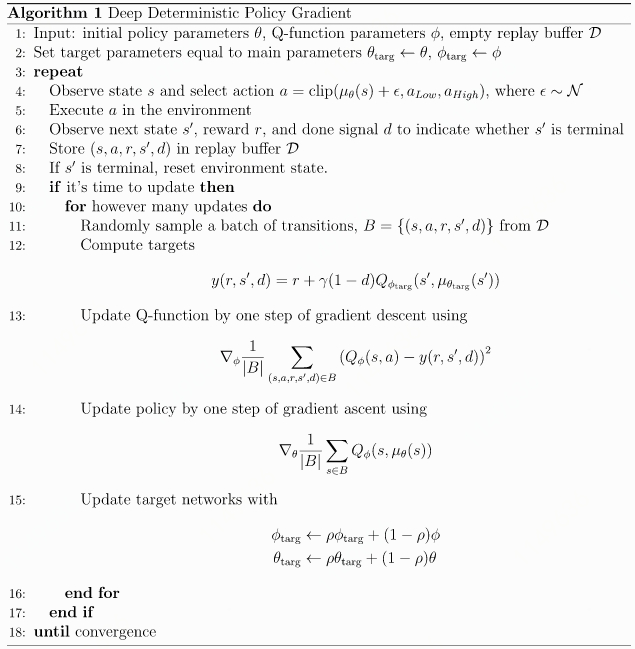Corresponding Code is modified from original OpenAI Spinning Up Git, but encapsulate all modules into a single file to faicilitate implementation and understanding:

import numpy as np
import tensorflow as tf
import gym
import time

def placeholder(dim=None):
    return tf.placeholder(dtype=tf.float32, shape=(None,dim) if dim else (None,))

def placeholders(*args):
    return [placeholder(dim) for dim in args]

def mlp(x, hidden_sizes=(32,), activation=tf.tanh, output_activation=None):
    for h in hidden_sizes[:-1]:
        x = tf.layers.dense(x, units=h, activation=activation)
    return tf.layers.dense(x, units=hidden_sizes[-1], activation=output_activation)

def get_vars(scope):
    return [x for x in tf.global_variables() if scope in x.name]

def count_vars(scope):
    v = get_vars(scope)
    return sum([np.prod(var.shape.as_list()) for var in v])

"""Actor-cirtics"""
def mlp_actor_critic(x, a, hidden_sizes=(256, 256), activation=tf.nn.relu,
                     output_activation=tf.tanh, action_space=None):
    act_dim = a.shape.as_list()[-1]
    act_limit = action_space.high[0]
    with tf.variable_scope('pi'):
        pi = act_limit * mlp(x, list(hidden_sizes)+[act_dim], activation, output_activation)
    with tf.variable_scope('q'):
        q = tf.squeeze(mlp(tf.concat([x,a], axis=-1), list(hidden_sizes)+[1], activation, None), axis=1)
    with tf.variable_scope('q', reuse=True):
        q_pi = tf.squeeze(mlp(tf.concat([x,pi], axis=-1), list(hidden_sizes)+[1], activation, None), axis=1)
    return pi, q, q_pi

class ReplayBuffer(object):
    """A simple FIFO experience replay buffer for DDPG agents. """

    def __init__(self, obs_dim, act_dim, size):
        self.obs1_buf = np.zeros([size, obs_dim], dtype=np.float32)
        self.obs2_buf = np.zeros([size, obs_dim], dtype=np.float32)
        self.acts_buf = np.zeros([size, act_dim], dtype=np.float32)
        self.rews_buf = np.zeros(size, dtype=np.float32)
        self.done_buf = np.zeros(size, dtype=np.float32)
        self.ptr, self.size, self.max_size = 0, 0, size

    def store(self, obs, act, rew, next_obs, done):
        self.obs1_buf[self.ptr] = obs
        self.obs2_buf[self.ptr] = next_obs
        self.acts_buf[self.ptr] = act
        self.rews_buf[self.ptr] = rew
        self.done_buf[self.ptr] = done
        self.ptr = (self.ptr+1) % self.max_size
        self.size = min(self.size+1, self.max_size)

    def sample_batch(self, batch_size=32):
        idxs = np.random.randint(0, self.size, size=batch_size)
        return dict(obs1=self.obs1_buf[idxs],
                    obs2=self.obs2_buf[idxs],
                    acts=self.acts_buf[idxs],
                    rews=self.rews_buf[idxs],
                    done=self.done_buf[idxs])

def ddpg(env_fn, actor_critic=mlp_actor_critic, ac_kwargs=dict(), seed=0, steps_per_epoch=4000, epochs=100,
         replay_size=int(1e6), gamma=0.99, polyak=0.995, pi_lr=1e-3, q_lr=1e-3, batch_size=100, start_steps=10000,
         update_after=1000, update_every=50, act_noise=0.1, num_test_episodes=10, max_ep_len=1000):
    """
    Deep Deterministic Policy Gradient (DDPG)
    env_fn: A function which creates a copy of the environment. The environment must satisfy the OpenAI Gym API.
    actor_critic: A function which takes in placeholder symbols for state, ``x_ph``, and action, ``a_ph``,
        and returns the main outputs from the agent's Tensorflow computation graph:
        ===========  ================  ======================================
        Symbol       Shape             Description
        ===========  ================  ======================================
        ``pi``       (batch, act_dim)  | Deterministically computes actions from policy given states.
        ``q``        (batch,)          | Gives the current estimate of Q* for
                                       | states in ``x_ph`` and actions in ``a_ph``.
        ``q_pi``     (batch,)          | Gives the composition of ``q`` and
                                       | ``pi`` for states in ``x_ph``: q(x, pi(x)).
        ===========  ================  ======================================
    ac_kwargs (dict): Any kwargs appropriate for the actor_critic function provided to DDPG.
    seed (int): Seed for random number generators.
    steps_per_epoch (int): Number of steps of interaction (state-action pairs)
        for the agent and the environment in each epoch.
    epochs (int): Number of epochs to run and train agent.
    replay_size (int): Maximum length of replay buffer.
    gamma (float): Discount factor. (Always between 0 and 1.)
    polyak (float): Interpolation factor in polyak averaging for target networks. Target networks are updated
        towards main networks according to:
        .. math:: \\theta_{\\text{targ}} \\leftarrow
            \\rho \\theta_{\\text{targ}} + (1-\\rho) \\theta
        where :math:`\\rho` is polyak. (Always between 0 and 1, usually close to 1.)
    pi_lr (float): Learning rate for policy.
    q_lr (float): Learning rate for Q-networks.
    batch_size (int): Minibatch size for SGD.
    start_steps (int):Number of steps for uniform-random action selection,before running real policy.Helps exploration.
    update_after (int): Number of env interactions to collect before starting to do gradient descent updates.
        Ensures replay buffer is full enough for useful updates.
    update_every (int): Number of env interactions that should elapse between gradient descent updates. Note:
        Regardless of how long you wait between updates, the ratio of env steps to gradient steps is locked to 1.
    act_noise (float): Stddev for Gaussian exploration noise added to policy at training time.
        (At test time, no noise is added.)
    num_test_episodes (int): Number of episodes to test the deterministic policy at the end of each epoch.
    max_ep_len (int): Maximum length of trajectory / episode / rollout.
    """
    tf.set_random_seed(seed)
    np.random.seed(seed)

    env, test_env = env_fn(), env_fn()
    obs_dim = env.observation_space.shape[0]
    act_dim = env.action_space.shape[0]

    # Action limit for clamping: critically, assumes all dimensions share the same bound!
    act_limit = env.action_space.high[0]

    # Share information about action space with policy architecture
    ac_kwargs['action_space'] = env.action_space

    # Inputs to computation graph
    x_ph, a_ph, x2_ph, r_ph, d_ph = placeholders(obs_dim, act_dim, obs_dim, None, None)

    # Main outputs from computation graph
    with tf.variable_scope('main'):
        pi, q, q_pi = actor_critic(x_ph, a_ph, **ac_kwargs)

    # Target networks
    with tf.variable_scope('target'):
        # Note that the action placeholder going to actor_critic here is
        # irrelevant, because we only need q_targ(s, pi_targ(s)).
        pi_targ, _, q_pi_targ = actor_critic(x2_ph, a_ph, **ac_kwargs)

    # Experience buffer
    replay_buffer = ReplayBuffer(obs_dim=obs_dim, act_dim=act_dim, size=replay_size)

    # Count variables
    var_counts = tuple(count_vars(scope) for scope in ['main/pi', 'main/q', 'main'])
    print('\nNumber of parameters: \t pi: %d, \t q: %d, \t total: %d\n'%var_counts)

    # Bellman backup for Q function
    backup = tf.stop_gradient(r_ph + gamma*(1-d_ph) * q_pi_targ)

    # DDPG losses
    pi_loss = -tf.reduce_mean(q_pi)
    q_loss = tf.reduce_mean((q - backup)**2)

    # Separate train ops for pi, q
    pi_optimizer = tf.train.AdamOptimizer(learning_rate=pi_lr)
    q_optimizer = tf.train.AdamOptimizer(learning_rate=q_lr)
    train_pi_op = pi_optimizer.minimize(pi_loss, var_list=get_vars('main/pi'))
    train_q_op = q_optimizer.minimize(q_loss, var_list=get_vars('main/q'))

    # Polyak averaging for target variables
    target_update = tf.group([tf.assign(v_targ, polyak*v_targ + (1-polyak)*v_main)
                              for v_main, v_targ in zip(get_vars('main'), get_vars('target'))])

    # Initializing targets to match main variables
    target_init = tf.group([tf.assign(v_targ, v_main)
                            for v_main, v_targ in zip(get_vars('main'), get_vars('target'))])

    sess = tf.Session()
    sess.run(tf.global_variables_initializer())
    sess.run(target_init)

    def get_action(o, noise_scale):
        a = sess.run(pi, feed_dict={x_ph: o.reshape(1,-1)})[0]
        a += noise_scale * np.random.randn(act_dim)
        return np.clip(a, -act_limit, act_limit)

    def test_agent():
        for j in range(num_test_episodes):
            o, d, ep_ret, ep_len = test_env.reset(), False, 0, 0
            while not(d or (ep_len==max_ep_len)):
                # Take deterministic actions at test time (noise_scale=0)
                o, r, d, _ = test_env.step(get_action(o, 0))
                ep_ret += r
                ep_len += 1
            print('#TestEpRet: {}, TestEpLen: {}'.format(ep_ret, ep_len))

    # Prepare for interaction with environment
    total_steps = steps_per_epoch * epochs
    # start_time = time.time()
    o, ep_ret, ep_len = env.reset(), 0, 0

    # Main loop: collect experience in env and update/log each epoch
    for t in range(total_steps):
        # Until start_steps have elapsed, randomly sample actions from a uniform distribution for
        # better exploration. Afterwards, use the learned policy (with some noise, via act_noise).
        if t > start_steps:
            a = get_action(o, act_noise)
        else:
            a = env.action_space.sample()

        # Step the env
        o2, r, d, _ = env.step(a)
        ep_ret += r
        ep_len += 1

        # Ignore the "done" signal if it comes from hitting the time horizon (that is, when it's an
        # artificial terminal signal that isn't based on the agent's state)
        d = False if ep_len==max_ep_len else d

        # Store experience to replay buffer
        replay_buffer.store(o, a, r, o2, d)

        # Super critical, easy to overlook step: make sure to update most recent observation!
        o = o2

        # End of trajectory handling
        if d or (ep_len == max_ep_len):
            print('#MainEpRet={}, MainEpLen={}'.format(ep_ret, ep_len))
            o, ep_ret, ep_len = env.reset(), 0, 0

        # Update handling
        if t >= update_after and t % update_every == 0:
            for _ in range(update_every):
                batch = replay_buffer.sample_batch(batch_size)
                feed_dict = {x_ph: batch['obs1'],
                             x2_ph: batch['obs2'],
                             a_ph: batch['acts'],
                             r_ph: batch['rews'],
                             d_ph: batch['done']}

                # Q-learning update
                outs = sess.run([q_loss, q, train_q_op], feed_dict)
                # print('LossQ={}, QVals={}'.format(outs[0], outs[1]))

                # Policy update
                outs = sess.run([pi_loss, train_pi_op, target_update], feed_dict)
                # print('LossPi={}'.format(outs[0]))

        # End of epoch wrap-up
        if (t + 1) % steps_per_epoch == 0:
            # epoch = (t + 1) // steps_per_epoch
            # Test the performance of the deterministic version of the agent.
            test_agent()

if __name__ == '__main__':
    # env = 'HalfCheetah-v2'
    env = 'MountainCarContinuous-v0'
    hid = 256
    l = 2
    gamma = 0.99
    seed = 0
    epochs = 50
    exp_name = 'ddpg'

    ddpg(lambda : gym.make(env), actor_critic=mlp_actor_critic, ac_kwargs=dict(hidden_sizes=[hid]*l),
         gamma=0.99, seed=seed, epochs=epochs)

100

101

102

103

104

105

106

107

108

109

110

111

112

113

114

115

116

117

118

119

120

121

122

123

124

125

126

127

128

129

130

131

132

133

134

135

136

137

138

139

140

141

142

143

144

145

146

147

148

149

150

151

152

153

154

155

156

157

158

159

160

161

162

163

164

165

166

167

168

169

170

171

172

173

174

175

176

177

178

179

180

181

182

183

184

185

186

187

188

189

190

191

192

193

194

195

196

197

198

199

200

201

202

203

204

205

206

207

208

209

210

211

212

213

214

215

216

217

218

219

220

221

222

223

224

225

226

227

228

229

230

231

232

233

234

235

236

237

238

239

240

241

242

243

244

245

246

247

248

249

import numpy as np

import tensorflow as tf

import gym

import time

def placeholder(dim=None):

return tf.placeholder(dtype=tf.float32, shape=(None,dim) if dim else (None,))

def placeholders(*args):

return [placeholder(dim) for dim in args]

def mlp(x, hidden_sizes=(32,), activation=tf.tanh, output_activation=None):

for h in hidden_sizes[:-1]:

x = tf.layers.dense(x, units=h, activation=activation)

return tf.layers.dense(x, units=hidden_sizes[-1], activation=output_activation)

def get_vars(scope):

return [x for x in tf.global_variables() if scope in x.name]

def count_vars(scope):

v = get_vars(scope)

return sum([np.prod(var.shape.as_list()) for var in v])

"""Actor-cirtics"""

def mlp_actor_critic(x, a, hidden_sizes=(256, 256), activation=tf.nn.relu,

output_activation=tf.tanh, action_space=None):

act_dim = a.shape.as_list()[-1]

act_limit = action_space.high[0]

with tf.variable_scope('pi'):

pi = act_limit * mlp(x, list(hidden_sizes)+[act_dim], activation, output_activation)

with tf.variable_scope('q'):

q = tf.squeeze(mlp(tf.concat([x,a], axis=-1), list(hidden_sizes)+[1], activation, None), axis=1)

with tf.variable_scope('q', reuse=True):

q_pi = tf.squeeze(mlp(tf.concat([x,pi], axis=-1), list(hidden_sizes)+[1], activation, None), axis=1)

return pi, q, q_pi

class ReplayBuffer(object):

"""A simple FIFO experience replay buffer for DDPG agents. """

def __init__(self, obs_dim, act_dim, size):

self.obs1_buf = np.zeros([size, obs_dim], dtype=np.float32)

self.obs2_buf = np.zeros([size, obs_dim], dtype=np.float32)

self.acts_buf = np.zeros([size, act_dim], dtype=np.float32)

self.rews_buf = np.zeros(size, dtype=np.float32)

self.done_buf = np.zeros(size, dtype=np.float32)

self.ptr, self.size, self.max_size = 0, 0, size

def store(self, obs, act, rew, next_obs, done):

self.obs1_buf[self.ptr] = obs

self.obs2_buf[self.ptr] = next_obs

self.acts_buf[self.ptr] = act

self.rews_buf[self.ptr] = rew

self.done_buf[self.ptr] = done

self.ptr = (self.ptr+1) % self.max_size

self.size = min(self.size+1, self.max_size)

def sample_batch(self, batch_size=32):

idxs = np.random.randint(0, self.size, size=batch_size)

return dict(obs1=self.obs1_buf[idxs],

obs2=self.obs2_buf[idxs],

acts=self.acts_buf[idxs],

rews=self.rews_buf[idxs],

done=self.done_buf[idxs])

def ddpg(env_fn, actor_critic=mlp_actor_critic, ac_kwargs=dict(), seed=0, steps_per_epoch=4000, epochs=100,

replay_size=int(1e6), gamma=0.99, polyak=0.995, pi_lr=1e-3, q_lr=1e-3, batch_size=100, start_steps=10000,

update_after=1000, update_every=50, act_noise=0.1, num_test_episodes=10, max_ep_len=1000):

"""

Deep Deterministic Policy Gradient (DDPG)

env_fn: A function which creates a copy of the environment. The environment must satisfy the OpenAI Gym API.

actor_critic: A function which takes in placeholder symbols for state, ``x_ph``, and action, ``a_ph``,

and returns the main outputs from the agent's Tensorflow computation graph:

=========== ================ ======================================

Symbol Shape Description

=========== ================ ======================================

``pi`` (batch, act_dim) | Deterministically computes actions from policy given states.

``q`` (batch,) | Gives the current estimate of Q* for

| states in ``x_ph`` and actions in ``a_ph``.

``q_pi`` (batch,) | Gives the composition of ``q`` and

| ``pi`` for states in ``x_ph``: q(x, pi(x)).

=========== ================ ======================================

ac_kwargs (dict): Any kwargs appropriate for the actor_critic function provided to DDPG.

seed (int): Seed for random number generators.

steps_per_epoch (int): Number of steps of interaction (state-action pairs)

for the agent and the environment in each epoch.

epochs (int): Number of epochs to run and train agent.

replay_size (int): Maximum length of replay buffer.

gamma (float): Discount factor. (Always between 0 and 1.)

polyak (float): Interpolation factor in polyak averaging for target networks. Target networks are updated

towards main networks according to:

.. math:: \\theta_{\\text{targ}} \\leftarrow

\\rho \\theta_{\\text{targ}} + (1-\\rho) \\theta

where :math:`\\rho` is polyak. (Always between 0 and 1, usually close to 1.)

pi_lr (float): Learning rate for policy.

q_lr (float): Learning rate for Q-networks.

batch_size (int): Minibatch size for SGD.

start_steps (int):Number of steps for uniform-random action selection,before running real policy.Helps exploration.

update_after (int): Number of env interactions to collect before starting to do gradient descent updates.

Ensures replay buffer is full enough for useful updates.

update_every (int): Number of env interactions that should elapse between gradient descent updates. Note:

Regardless of how long you wait between updates, the ratio of env steps to gradient steps is locked to 1.

act_noise (float): Stddev for Gaussian exploration noise added to policy at training time.

(At test time, no noise is added.)

num_test_episodes (int): Number of episodes to test the deterministic policy at the end of each epoch.

max_ep_len (int): Maximum length of trajectory / episode / rollout.

"""

tf.set_random_seed(seed)

np.random.seed(seed)

env, test_env = env_fn(), env_fn()

obs_dim = env.observation_space.shape[0]

act_dim = env.action_space.shape[0]

# Action limit for clamping: critically, assumes all dimensions share the same bound!

act_limit = env.action_space.high[0]

# Share information about action space with policy architecture

ac_kwargs['action_space'] = env.action_space

# Inputs to computation graph

x_ph, a_ph, x2_ph, r_ph, d_ph = placeholders(obs_dim, act_dim, obs_dim, None, None)

# Main outputs from computation graph

with tf.variable_scope('main'):

pi, q, q_pi = actor_critic(x_ph, a_ph, **ac_kwargs)

# Target networks

with tf.variable_scope('target'):

# Note that the action placeholder going to actor_critic here is

# irrelevant, because we only need q_targ(s, pi_targ(s)).

pi_targ, _, q_pi_targ = actor_critic(x2_ph, a_ph, **ac_kwargs)

# Experience buffer

replay_buffer = ReplayBuffer(obs_dim=obs_dim, act_dim=act_dim, size=replay_size)

# Count variables

var_counts = tuple(count_vars(scope) for scope in ['main/pi', 'main/q', 'main'])

print('\nNumber of parameters: \t pi: %d, \t q: %d, \t total: %d\n'%var_counts)

# Bellman backup for Q function

backup = tf.stop_gradient(r_ph + gamma*(1-d_ph) * q_pi_targ)

# DDPG losses

pi_loss = -tf.reduce_mean(q_pi)

q_loss = tf.reduce_mean((q - backup)**2)

# Separate train ops for pi, q

pi_optimizer = tf.train.AdamOptimizer(learning_rate=pi_lr)

q_optimizer = tf.train.AdamOptimizer(learning_rate=q_lr)

train_pi_op = pi_optimizer.minimize(pi_loss, var_list=get_vars('main/pi'))

train_q_op = q_optimizer.minimize(q_loss, var_list=get_vars('main/q'))

# Polyak averaging for target variables

target_update = tf.group([tf.assign(v_targ, polyak*v_targ + (1-polyak)*v_main)

for v_main, v_targ in zip(get_vars('main'), get_vars('target'))])

# Initializing targets to match main variables

target_init = tf.group([tf.assign(v_targ, v_main)

for v_main, v_targ in zip(get_vars('main'), get_vars('target'))])

sess = tf.Session()

sess.run(tf.global_variables_initializer())

sess.run(target_init)

def get_action(o, noise_scale):

a = sess.run(pi, feed_dict={x_ph: o.reshape(1,-1)})[0]

a += noise_scale * np.random.randn(act_dim)

return np.clip(a, -act_limit, act_limit)

def test_agent():

for j in range(num_test_episodes):

o, d, ep_ret, ep_len = test_env.reset(), False, 0, 0

while not(d or (ep_len==max_ep_len)):

# Take deterministic actions at test time (noise_scale=0)

o, r, d, _ = test_env.step(get_action(o, 0))

ep_ret += r

ep_len += 1

print('#TestEpRet: {}, TestEpLen: {}'.format(ep_ret, ep_len))

# Prepare for interaction with environment

total_steps = steps_per_epoch * epochs

# start_time = time.time()

o, ep_ret, ep_len = env.reset(), 0, 0

# Main loop: collect experience in env and update/log each epoch

for t in range(total_steps):

# Until start_steps have elapsed, randomly sample actions from a uniform distribution for

# better exploration. Afterwards, use the learned policy (with some noise, via act_noise).

if t > start_steps:

a = get_action(o, act_noise)

else:

a = env.action_space.sample()

# Step the env

o2, r, d, _ = env.step(a)

ep_ret += r

ep_len += 1

# Ignore the "done" signal if it comes from hitting the time horizon (that is, when it's an

# artificial terminal signal that isn't based on the agent's state)

d = False if ep_len==max_ep_len else d

# Store experience to replay buffer

replay_buffer.store(o, a, r, o2, d)

# Super critical, easy to overlook step: make sure to update most recent observation!

o = o2

# End of trajectory handling

if d or (ep_len == max_ep_len):

print('#MainEpRet={}, MainEpLen={}'.format(ep_ret, ep_len))

o, ep_ret, ep_len = env.reset(), 0, 0

# Update handling

if t >= update_after and t % update_every == 0:

for _ in range(update_every):

batch = replay_buffer.sample_batch(batch_size)

feed_dict = {x_ph: batch['obs1'],

x2_ph: batch['obs2'],

a_ph: batch['acts'],

r_ph: batch['rews'],

d_ph: batch['done']}

# Q-learning update

outs = sess.run([q_loss, q, train_q_op], feed_dict)

# print('LossQ={}, QVals={}'.format(outs[0], outs[1]))

# Policy update

outs = sess.run([pi_loss, train_pi_op, target_update], feed_dict)

# print('LossPi={}'.format(outs[0]))

# End of epoch wrap-up

if (t + 1) % steps_per_epoch == 0:

# epoch = (t + 1) // steps_per_epoch

# Test the performance of the deterministic version of the agent.

test_agent()

if __name__ == '__main__':

# env = 'HalfCheetah-v2'

env = 'MountainCarContinuous-v0'

hid = 256

l = 2

gamma = 0.99

seed = 0

epochs = 50

exp_name = 'ddpg'

ddpg(lambda : gym.make(env), actor_critic=mlp_actor_critic, ac_kwargs=dict(hidden_sizes=[hid]*l),

gamma=0.99, seed=seed, epochs=epochs)

The result is as follow: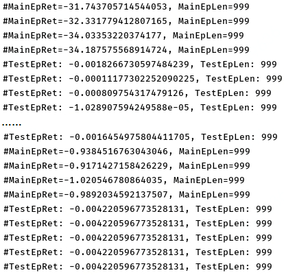

Version 2
I draw a diagram to illustarte the iteration process: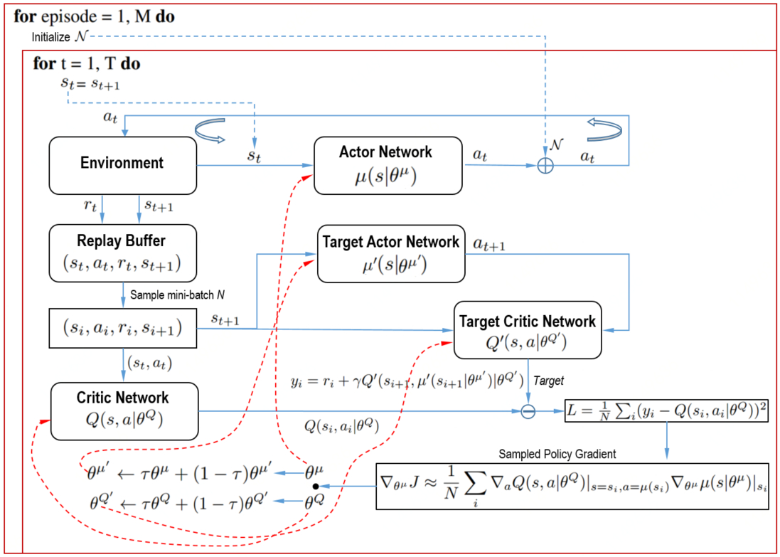
DDPG alogrithm pseudocode from original DDPG paper and correspondng a minimal implementation:

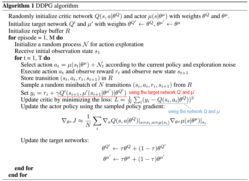
Code implementation

import gym
import random
import collections
import torch
import torch.nn as nn
import torch.nn.functional as F
import torch.optim as optim
import numpy as np

lr_mu = 0.0005
lr_q = 0.001
gamma = 0.99
batch_size = 32
buffer_limit = 50000
tau = 0.005 # for target network soft update

class ReplayBuffer(object):
    def __init__(self):
        self.buffer = collections.deque(maxlen=buffer_limit)

    def put(self, transition):
        self.buffer.append(transition)

    def sample(self, n):
        mini_batch = random.sample(self.buffer, n)
        s_lst, a_lst, r_lst, s_prime_lst, done_mask_lst = [], [], [], [], []

        for transition in mini_batch:
            s, a, r, s_prime, done_mask = transition
            s_lst.append(s)
            a_lst.append([a])
            r_lst.append([r])
            s_prime_lst.append(s_prime)
            done_mask_lst.append([done_mask])

        return torch.tensor(s_lst, dtype=torch.float), torch.tensor(a_lst), torch.tensor(r_lst), \
               torch.tensor(s_prime_lst, dtype=torch.float), torch.tensor(done_mask_lst)

    def size(self):
        return len(self.buffer)

class MuNet(nn.Module):
    def __init__(self):
        super(MuNet, self).__init__()
        self.fc1 = nn.Linear(3, 128)
        self.fc2 = nn.Linear(128, 64)
        self.fc_mu = nn.Linear(64, 1)

    def forward(self, x):
        x = F.relu(self.fc1(x))
        x = F.relu(self.fc2(x))
        mu = torch.tanh(self.fc_mu(x))*2 # Multipled by 2 because the action space of the Pendulum-v0 is [-2,2]
        return mu

class QNet(nn.Module):
    def __init__(self):
        super(QNet, self).__init__()
        self.fc_s = nn.Linear(3, 64)
        self.fc_a = nn.Linear(1, 64)
        self.fc_q = nn.Linear(128, 32)
        self.fc_3 = nn.Linear(32, 1)

    def forward(self, x, a):
        h1 = F.relu(self.fc_s(x))
        h2 = F.relu(self.fc_a(a))
        cat = torch.cat([h1, h2], dim=1)
        q = F.relu(self.fc_q(cat))
        q = self.fc_3(q)
        return q

class OrnsteinUhlenbeckNoise(object):

    def __init__(self, mu):
        self.theta, self.dt, self.sigma = 0.1, 0.01, 0.1
        self.mu = mu
        self.x_prev = np.zeros_like(self.mu)

    def __call__(self):
        x = self.x_prev + self.theta * (self.mu - self.x_prev) * self.dt + \
            self.sigma * np.sqrt(self.dt) * np.random.normal(size=self.mu.shape)
        self.x_prev = x
        return x

def train(mu, mu_target, q, q_target, memory, q_optimizer, mu_optimizer):

    s, a, r, s_prime, done_mask = memory.sample(batch_size)

    target = r + gamma * q_target(s_prime, mu_target(s_prime))
    q_loss = F.smooth_l1_loss(q(s,a), target.detach())
    q_optimizer.zero_grad()
    q_loss.backward()
    q_optimizer.step()

    mu_loss = -q(s, mu(s)).mean()
    mu_optimizer.zero_grad()
    mu_loss.backward()
    mu_optimizer.step()

def soft_update(net, net_target):
    for param_target, param in zip(net_target.parameters(), net.parameters()):
        param_target.data.copy_(param_target.data * (1.0 - tau) + param.data * tau)

def main():
    env = gym.make('Pendulum-v0')
    memory = ReplayBuffer()

    q, q_target = QNet(), QNet()
    q_target.load_state_dict(q.state_dict())
    mu, mu_target = MuNet(), MuNet()
    mu_target.load_state_dict(mu.state_dict())

    score = 0.0
    print_interval = 20

    mu_optimizer = optim.Adam(mu.parameters(), lr=lr_mu)
    q_optimizer = optim.Adam(q.parameters(), lr=lr_q)
    ou_noise = OrnsteinUhlenbeckNoise(mu=np.zeros(1))

    for n_epi in range(10000):
        s = env.reset()

        for t in range(300):
            a = mu(torch.from_numpy(s).float())
            a = a.item() + ou_noise()[0]
            s_prime, r, done, info = env.step([a])
            memory.put((s, a, r/100.0, s_prime, done))
            score += r
            s = s_prime

            if done:
                break

        if memory.size()>2000:
            for i in range(10):
                train(mu, mu_target, q, q_target, memory, q_optimizer, mu_optimizer)
                soft_update(mu, mu_target)
                soft_update(q, q_target)

        if n_epi%print_interval==0 and n_epi!=0:
            print('# of episode :{}, avg score: {:.1f}'.format(n_epi, score/print_interval))
            score = 0.0
    env.close()

if __name__ == '__main__':
    main()

100

101

102

103

104

105

106

107

108

109

110

111

112

113

114

115

116

117

118

119

120

121

122

123

124

125

126

127

128

129

130

131

132

133

134

135

136

137

138

139

140

141

142

143

144

145

import gym

import random

import collections

import torch

import torch.nn as nn

import torch.nn.functional as F

import torch.optim as optim

import numpy as np

lr_mu = 0.0005

lr_q = 0.001

gamma = 0.99

batch_size = 32

buffer_limit = 50000

tau = 0.005 # for target network soft update

class ReplayBuffer(object):

def __init__(self):

self.buffer = collections.deque(maxlen=buffer_limit)

def put(self, transition):

self.buffer.append(transition)

def sample(self, n):

mini_batch = random.sample(self.buffer, n)

s_lst, a_lst, r_lst, s_prime_lst, done_mask_lst = [], [], [], [], []

for transition in mini_batch:

s, a, r, s_prime, done_mask = transition

s_lst.append(s)

a_lst.append([a])

r_lst.append([r])

s_prime_lst.append(s_prime)

done_mask_lst.append([done_mask])

return torch.tensor(s_lst, dtype=torch.float), torch.tensor(a_lst), torch.tensor(r_lst), \

torch.tensor(s_prime_lst, dtype=torch.float), torch.tensor(done_mask_lst)

def size(self):

return len(self.buffer)

class MuNet(nn.Module):

def __init__(self):

super(MuNet, self).__init__()

self.fc1 = nn.Linear(3, 128)

self.fc2 = nn.Linear(128, 64)

self.fc_mu = nn.Linear(64, 1)

def forward(self, x):

x = F.relu(self.fc1(x))

x = F.relu(self.fc2(x))

mu = torch.tanh(self.fc_mu(x))*2 # Multipled by 2 because the action space of the Pendulum-v0 is [-2,2]

return mu

class QNet(nn.Module):

def __init__(self):

super(QNet, self).__init__()

self.fc_s = nn.Linear(3, 64)

self.fc_a = nn.Linear(1, 64)

self.fc_q = nn.Linear(128, 32)

self.fc_3 = nn.Linear(32, 1)

def forward(self, x, a):

h1 = F.relu(self.fc_s(x))

h2 = F.relu(self.fc_a(a))

cat = torch.cat([h1, h2], dim=1)

q = F.relu(self.fc_q(cat))

q = self.fc_3(q)

return q

class OrnsteinUhlenbeckNoise(object):

def __init__(self, mu):

self.theta, self.dt, self.sigma = 0.1, 0.01, 0.1

self.mu = mu

self.x_prev = np.zeros_like(self.mu)

def __call__(self):

x = self.x_prev + self.theta * (self.mu - self.x_prev) * self.dt + \

self.sigma * np.sqrt(self.dt) * np.random.normal(size=self.mu.shape)

self.x_prev = x

return x

def train(mu, mu_target, q, q_target, memory, q_optimizer, mu_optimizer):

s, a, r, s_prime, done_mask = memory.sample(batch_size)

target = r + gamma * q_target(s_prime, mu_target(s_prime))

q_loss = F.smooth_l1_loss(q(s,a), target.detach())

q_optimizer.zero_grad()

q_loss.backward()

q_optimizer.step()

mu_loss = -q(s, mu(s)).mean()

mu_optimizer.zero_grad()

mu_loss.backward()

mu_optimizer.step()

def soft_update(net, net_target):

for param_target, param in zip(net_target.parameters(), net.parameters()):

param_target.data.copy_(param_target.data * (1.0 - tau) + param.data * tau)

def main():

env = gym.make('Pendulum-v0')

memory = ReplayBuffer()

q, q_target = QNet(), QNet()

q_target.load_state_dict(q.state_dict())

mu, mu_target = MuNet(), MuNet()

mu_target.load_state_dict(mu.state_dict())

score = 0.0

print_interval = 20

mu_optimizer = optim.Adam(mu.parameters(), lr=lr_mu)

q_optimizer = optim.Adam(q.parameters(), lr=lr_q)

ou_noise = OrnsteinUhlenbeckNoise(mu=np.zeros(1))

for n_epi in range(10000):

s = env.reset()

for t in range(300):

a = mu(torch.from_numpy(s).float())

a = a.item() + ou_noise()[0]

s_prime, r, done, info = env.step([a])

memory.put((s, a, r/100.0, s_prime, done))

score += r

s = s_prime

if done:

break

if memory.size()>2000:

for i in range(10):

train(mu, mu_target, q, q_target, memory, q_optimizer, mu_optimizer)

soft_update(mu, mu_target)

soft_update(q, q_target)

if n_epi%print_interval==0 and n_epi!=0:

print('# of episode :{}, avg score: {:.1f}'.format(n_epi, score/print_interval))

score = 0.0

env.close()

if __name__ == '__main__':

main()

The result is as follow: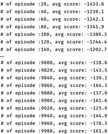

4. Reference

1. Continuous Control With Deep Reinforcement Learning, Lillicrap et al. 2016
2. OpenAI Spinning Up Documentation, DDPG

1. DDPG Overview

2. Formulation

3. Pseudocode and Code Implementation

4. Reference

Leave a Reply Cancel reply