Dynamic Programming in Reinforcement Learning

Dynamic Programming (DP) plays an important role in traditional approaches of solving reinforcement learning with known dynamics. This post focuses on a more classical view of the basic reinforcment learning solution, mostly the tabular case.

We take an overview of the dynamic programming problem, followed by the solution of DP problems, namely, policy search, policy iteration and value iteration, along with the basic process of policy evaluation and policy improvement, to faciliate understanding, both theroy and code examples are presented.

1. Dynamic Programming Overview

The term dynamic programming (DP) refers to a collection of algorithms that can be used to compute optimal policies given a perfect model of the environment as a Markov decision process (MDP). Classical DP algorithms are of limited utility in reinforcement learning both because of their assumption of a perfect model and because of their great computational expense.
Dynamic Programming or (DP) is a method for solving complex problems by breaking them down into sub problems, solve the sub problems, and combine solutions to the sub problems to solve the overall problem.
DP is a very general solution method for problems which have two properties, the first is “optimal substructure” where the principle of optimality applies (discussed later). It tells us that we can solve some overall problem by breaking it down into two or more pieces, solve for each of the pieces, and the optimal solution to the pieces tells us how to get the optimal solution to the overall problem.
E.g. if your problem is to get from some point in space to the nearest wall, you will try to figure out the shortest path to the wall. DP tells us that the shortest path to the wall is the shortest path to a midpoint between you and the wall combined with the shortest path from that midpoint to the wall.
The second property is “overlapping sub problems”, which means that the sub problems which occur once, will occur again and again. We broke down the problem of getting to the wall into first getting to the midpoint, and then getting to the wall. That will help us solve the sub problem of how to get from another point to the wall. Solutions can be cached and reused.
Markov Decision Processes satisfy both mentioned properties. Bellman equation gives us recursive decomposition (the first property). Bellman equation tells us how to break down the optimal value function into two pieces, the optimal behavior for one step followed by the optimal behavior after that step.
What gives us the overlapping sub problems property in MDPs is the value function. It’s like a cache of the good information we figured out about the MDP.

2. Solving DP Problems

Three methods are commonly used to solve the DP problems with known dynamics/models, including policy search, policy iteration (characterized by the policy evaluation intertwining with the policy improvement) and value iteration. As illustrated in the following figure: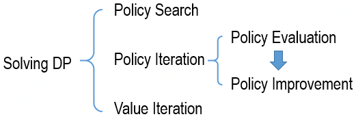
As most of the solutions are based on policy evaluation and policy improvement, I will introduce them first regardless of the order in the figure.

2.1 Policy Evaluation

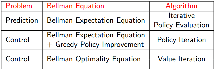
In policy evaluation, we’re given an MDP and a policy $\pi$ . We try to evaluate the given policy. We can evaluate the given policy through iterative application of Bellman expectation equation, and later use the Bellman optimality equation to do control.
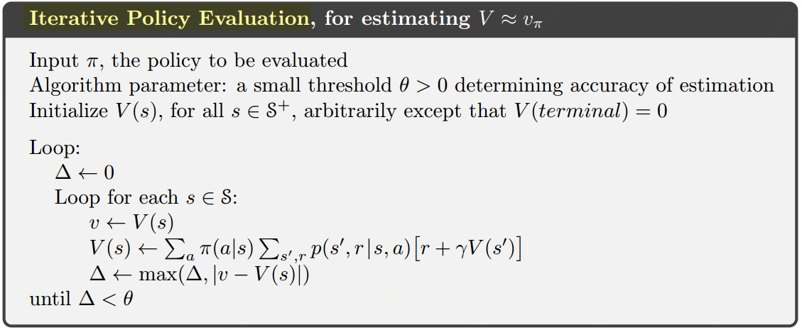
How to compute the state-value function $v_{\pi}$ for an arbitrary policy $\pi$ . This is called policy evaluation in the DP literature, or prediction problem.

$\begin{array}{l}{v_{\rm{\pi }}}\left( s \right) \buildrel\textstyle.\over= {\mathbb{E}_{\rm{\pi }}}\left[ {{G_t}\left| {{S_t} = s} \right.} \right]\\\;\;\;\;\;\;\;\;{\kern 1pt} = {\mathbb{E}_{\rm{\pi }}}\left[ {{R_{t + 1}} + \gamma {G_{t + 1}}\left| {{S_t} = s} \right.} \right]\\\;\;\;\;\;\;\;\;{\kern 1pt} = {\mathbb{E}_{\rm{\pi }}}\left[ {{R_{t + 1}} + \gamma {v_{\rm{\pi }}}\left( {{S_{t + 1}}} \right)\left| {{S_t} = s} \right.} \right]\\\;\;\;\;\;\;\;\;{\kern 1pt} = \sum\limits_a {{\rm{\pi }}\left( {a\left| s \right.} \right)} \sum\limits_{s',r} {p\left( {s',r\left| {s,a} \right.} \right)} \left[ {r + \gamma {v_{\rm{\pi }}}\left( {s'} \right)} \right]\end{array}$

If the environment’s dynamics are completely known, then above equation is a system of $\left| S \right|$ simultaneous linear equations with $\left| S \right|$ unknowns (the ${v_{\rm{\pi }}}\left( s \right),s \in S$ ). The analytical solution may cost much computation. An iterative method is most suitable. Consider a sequence of approximate value functions ${v_0},{v_1},{v_2}, \cdots$ , each mapping ${S^ + }$ to $\mathcal{R}$ (the real numbers). The initial approximation, $v_0$ , is chosen arbitrarily (except that the terminal state, if any, must be given value 0), and each successive approximation is obtained by using the Bellman equation for ${v_{\rm{\pi }}}$ as an update rule:

$\begin{array}{l}{v_{k{\rm{ + 1}}}}\left( s \right) \buildrel\textstyle.\over= {\mathbb{E}_{\rm{\pi }}}\left[ {{R_{t + 1}} + \gamma {v_{\rm{\pi }}}\left( {{S_{t + 1}}} \right)\left| {{S_t} = s} \right.} \right]\\{\kern 1pt} {\kern 1pt} {\kern 1pt} {\kern 1pt} {\kern 1pt} {\kern 1pt} \;\;\;\;\;\;\;\;{\kern 1pt} = \sum\limits_a {{\rm{\pi }}\left( {a\left| s \right.} \right)} \sum\limits_{s',r} {p\left( {s',r\left| {s,a} \right.} \right)} \left[ {r + \gamma {v_k}\left( {s'} \right)} \right]\end{array}$

for all $s \in S$ .
Expected update: To produce each successive approximation, ${v_{k{\rm{ + 1}}}}$ from ${{v_k}}$ , iterative policy evaluation applies the same operation to each state $s$ : it replaces the old value of $s$ with a new value obtained from the old values of the successor states of $s$ , and the expected immediate rewards, along all the one-step transitions possible under the policy being evaluated. Each iteration of iterative policy evaluation updates the value of every state once to produce the new approximate value function ${v_{k{\rm{ + 1}}}}$ . All the updates done in DP algorithms are called expected updates because they are based on an expectation over all possible next states rather than on a sample next state.
There are two versions of policy evaluation, as below:

One array in-place version:

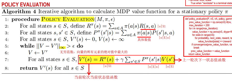Corresponding Bellman backup diagram is as follow:

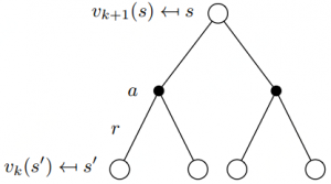In formula, it would be:

$\begin{array}{l}{v_{k{\rm{ + 1}}}}\left( s \right) = \sum\limits_{a \in \mathcal{A}} {{\rm{\pi }}\left( {a\left| s \right.} \right)\left( {\mathcal{R}_s^a + \gamma \sum\limits_{s' \in S} {\mathcal{P}_{ss'}^a{v_k}\left( {s'} \right)} } \right)} \\{{\bf{v}}^{k + 1}} = {{\bf{\mathcal{R}}}^{\bf{\pi }}} + \gamma {{\bf{\mathcal{P}}}^{\bf{\pi }}}{{\bf{v}}^k}\end{array}$

$\mathcal{R}_s^a$ is the immediate reward correlating to state. Analytical solution can be calculated by the second formula.
Define the value function at next iteration by plugging in the previous iterations values of the leaves to effectively take the value functions from the last iteration BK, we plug in those values in the leaves, we back up those values to compute one single new value for the next iteration of the root. So we figure out the $k+1$ by looking one-step ahead from value function of last iteration.
The following is an example to illustrate the calculation process.

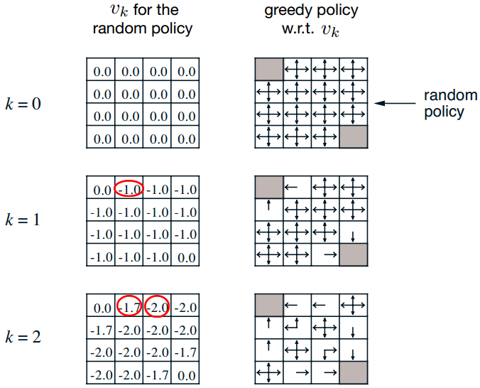
Calculation process is as follow:
When k=1,
   -1.0 = 0.25*(-1+0) + 0.25*(-1+0) + 0.25*(-1+0) + 0.25*(-1+0)
When k=2,
   -1.7 = 0.25*(-1+0) + 0.25*(-1-1) + 0.25*(-1-1) + 0.25*(-1-1)
   -2.0 = 0.25*(-1-1) + 0.25*(-1-1.0) + 0.25*(-1-1.0) + 0.25*(-1-1.0)
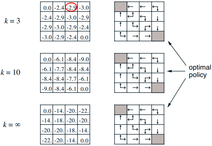
When k=3,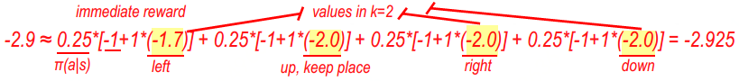
A more detailed view drawn from other author is,

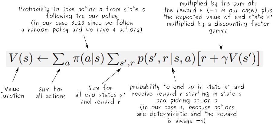
Code implementation for policy evaluation is as follow:

def policy_evaluation(P, nS, nA, policy, gamma=0.9, tol=1e-3):
    """Evaluate the value function from a given policy.

    Parameters
    ----------
    P, nS, nA, gamma:
        defined at beginning of file
    policy: np.array[nS]
        The policy to evaluate. Maps states to actions.
    tol: float
        Terminate policy evaluation when
            max |value_function(s) - prev_value_function(s)| < tol
    Returns
    -------
    value_function: np.ndarray[nS]
        The value function of the given policy, where value_function[s] is
        the value of state s
    """

    value_function = np.zeros(nS)

    while True:
        # new value function
        new_value_function = np.zeros(nS)

        # loop over state
        for s in range(nS):
            # To accumelate bellman expectation eqn with respect to actions
            for a in range(nA):
                # get transitions
                [(prob, next_state, reward, done)] = P[s][a]
                # apply bellman expectatoin eqn
                # Here assuming action_prob = 0.25, can also get from policy
                new_value_function[s] += 0.25 * prob * (reward + gamma * value_function[next_state])

        delta = np.max(np.abs(new_value_function - value_function))
        # the new value function
        value_function = new_value_function
        if delta < tol:
            break
    return value_function

def policy_evaluation(P, nS, nA, policy, gamma=0.9, tol=1e-3):

"""Evaluate the value function from a given policy.

Parameters

----------

P, nS, nA, gamma:

defined at beginning of file

policy: np.array[nS]

The policy to evaluate. Maps states to actions.

tol: float

Terminate policy evaluation when

max |value_function(s) - prev_value_function(s)| < tol

Returns

-------

value_function: np.ndarray[nS]

The value function of the given policy, where value_function[s] is

the value of state s

"""

value_function = np.zeros(nS)

while True:

# new value function

new_value_function = np.zeros(nS)

# loop over state

for s in range(nS):

# To accumelate bellman expectation eqn with respect to actions

for a in range(nA):

# get transitions

[(prob, next_state, reward, done)] = P[s][a]

# apply bellman expectatoin eqn

# Here assuming action_prob = 0.25, can also get from policy

new_value_function[s] += 0.25 * prob * (reward + gamma * value_function[next_state])

delta = np.max(np.abs(new_value_function - value_function))

# the new value function

value_function = new_value_function

if delta < tol:

break

return value_function

Take the Gridworld Example from “Nuts & Bolts of Reinforcement Learning: Model Based Planning using Dynamic Programming”

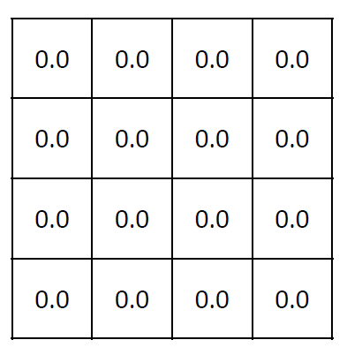
Similarly, for all non-terminal states, $v_{1}(s) = -1$ .
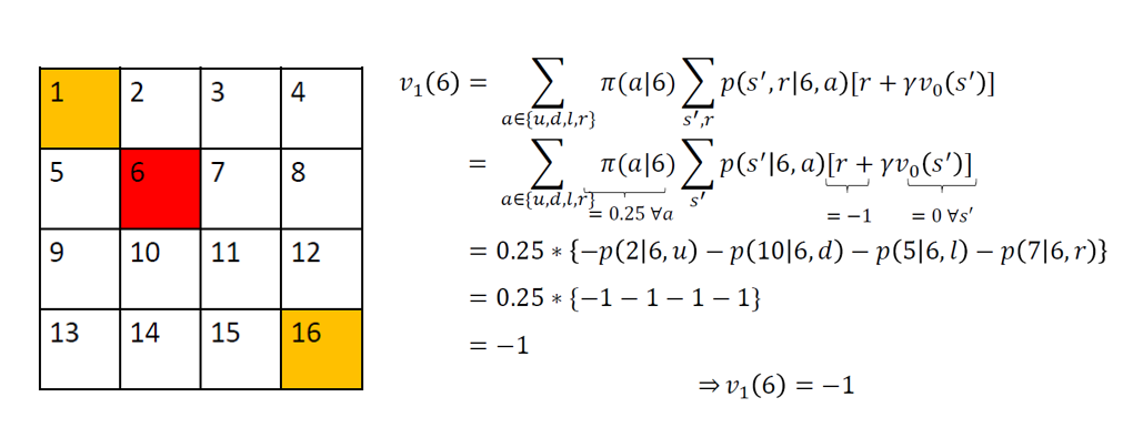
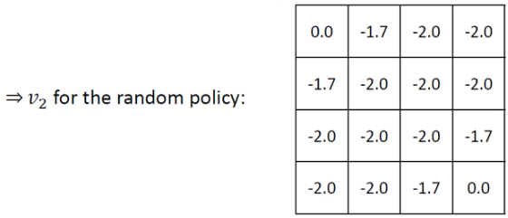
For terminal states $p\left( {s'\left| {s,a} \right.} \right) = 0$ and hence ${v_k}(1) = {v_k}(16) = 0$ for all $k$ . So v1 for the random policy is given by:

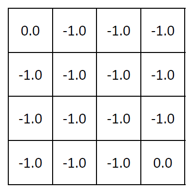
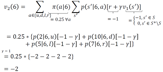
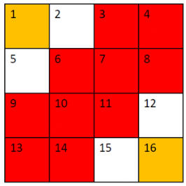
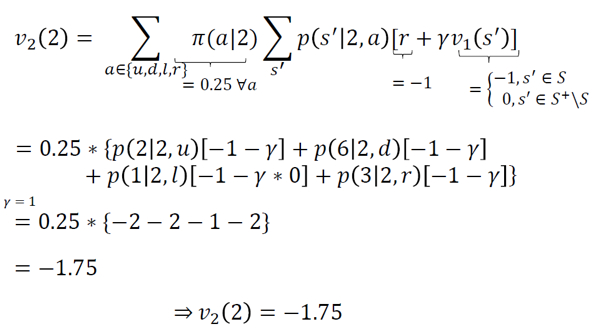
For all the remaining states, i.e., 2, 5, 12 and 15, $v_2$ can be calculated as follows:

2.2 Policy Improvement

Policy Improvement: the process of making a new policy that improves on an original policy, by making it greedy with respect to the value function of the original policy.

$\begin{array}{l}{\rm{\pi '}}\left( s \right) \buildrel\textstyle.\over= \mathop {\arg \max }\limits_a {q_{\rm{\pi }}}\left( {s,a} \right)\\\;\;{\kern 1pt} {\kern 1pt} {\kern 1pt} {\kern 1pt} {\kern 1pt} {\kern 1pt} {\kern 1pt} {\kern 1pt} {\kern 1pt} {\kern 1pt} {\kern 1pt} {\kern 1pt} {\kern 1pt} {\kern 1pt} {\kern 1pt} {\kern 1pt} {\kern 1pt} {\kern 1pt} {\kern 1pt} {\kern 1pt} = \mathop {\arg \max }\limits_a \mathbb{E}\left[ {{R_{t + 1}} + \gamma {v_{\rm{\pi }}}\left( {{S_{t + 1}}} \right)\left| {{S_t} = s,{A_t} = a} \right.} \right]\\\;\;{\kern 1pt} {\kern 1pt} {\kern 1pt} {\kern 1pt} {\kern 1pt} {\kern 1pt} {\kern 1pt} {\kern 1pt} {\kern 1pt} {\kern 1pt} {\kern 1pt} {\kern 1pt} {\kern 1pt} {\kern 1pt} {\kern 1pt} {\kern 1pt} {\kern 1pt} {\kern 1pt} {\kern 1pt} {\kern 1pt} = \mathop {\mathop {\arg \max }\limits_a \sum\limits_{s',r} {p\left( {s',r\left| {s,a} \right.} \right)\left[ {r + \gamma {v_{\rm{\pi }}}\left( {s'} \right)} \right]} }\limits_a \end{array}$

Corresponding algorithm is:

Code implementation for policy improvement algorithm is as follow.

def policy_improvement(P, nS, nA, value_from_policy, policy, gamma=0.9):
    """Given the value function from policy improve the policy.

    Parameters
    ----------
    P, nS, nA, gamma:
        defined at beginning of file
    value_from_policy: np.ndarray
        The value calculated from the policy
    policy: np.array
        The previous policy.

    Returns
    -------
    new_policy: np.ndarray[nS]
        An array of integers. Each integer is the optimal action to take
        in that state according to the environment dynamics and the
        given value function.
    """
    new_policy = np.zeros(nS, dtype='int')
    for s in range(nS):
        action_reward = []
        for a in range(nA):
            prob, next_state, reward, done = P[s][a][0]
            action_reward.append(reward + gamma * prob * value_from_policy[next_state])
        new_policy[s] = np.argmax(action_reward)
    return new_policy

def policy_improvement(P, nS, nA, value_from_policy, policy, gamma=0.9):

"""Given the value function from policy improve the policy.

Parameters

----------

P, nS, nA, gamma:

defined at beginning of file

value_from_policy: np.ndarray

The value calculated from the policy

policy: np.array

The previous policy.

Returns

-------

new_policy: np.ndarray[nS]

An array of integers. Each integer is the optimal action to take

in that state according to the environment dynamics and the

given value function.

"""

new_policy = np.zeros(nS, dtype='int')

for s in range(nS):

action_reward = []

for a in range(nA):

prob, next_state, reward, done = P[s][a][0]

action_reward.append(reward + gamma * prob * value_from_policy[next_state])

new_policy[s] = np.argmax(action_reward)

return new_policy

2.3 Policy Iteration

The reason for computing the value function for a policy is to help find better policies.
A finite MDP has only a finite number of policies, this process must converge to an optimal policy and optimal value function in a finite number of iterations. The policy iteration is shown in the following box.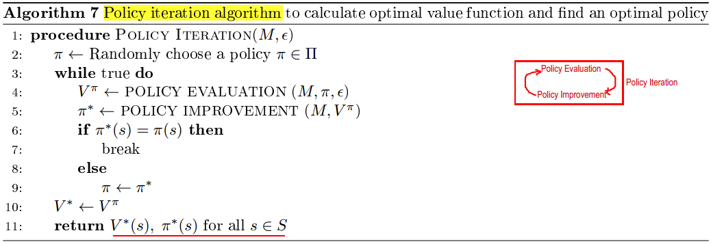

In combination with above policy evaluation and improvement process, code implementation for policy iteration algorithm is.

def policy_iteration(P, nS, nA, gamma=0.9, tol=10e-3):
    """Runs policy iteration.

    You should call the policy_evaluation() and policy_improvement() methods to
    implement this method.

    Parameters
    ----------
    P, nS, nA, gamma:
        defined at beginning of file
    tol: float
        tol parameter used in policy_evaluation()
    Returns:
    ----------
    value_function: np.ndarray[nS]
    policy: np.ndarray[nS]
    """

    # value_function = np.zeros(nS)
    policy = np.zeros(nS, dtype=int)

    while True:
        value_function = policy_evaluation(P, nS, nA, policy, gamma, tol)
        new_policy = policy_improvement(P, nS, nA, value_function, policy, gamma)
        policy_change = (new_policy != policy).sum()
        policy = new_policy
        if policy_change == 0:
            break
    return value_function, policy

def policy_iteration(P, nS, nA, gamma=0.9, tol=10e-3):

"""Runs policy iteration.

You should call the policy_evaluation() and policy_improvement() methods to

implement this method.

Parameters

----------

P, nS, nA, gamma:

defined at beginning of file

tol: float

tol parameter used in policy_evaluation()

Returns:

----------

value_function: np.ndarray[nS]

policy: np.ndarray[nS]

"""

# value_function = np.zeros(nS)

policy = np.zeros(nS, dtype=int)

while True:

value_function = policy_evaluation(P, nS, nA, policy, gamma, tol)

new_policy = policy_improvement(P, nS, nA, value_function, policy, gamma)

policy_change = (new_policy != policy).sum()

policy = new_policy

if policy_change == 0:

break

return value_function, policy

2.4 Value Iteration

One drawback to policy iteration is that each of its iterations involves policy evaluation, which may itself be a protracted iterative computation requiring multiple sweeps through the state set.
The policy evaluation step of policy iteration can be truncated in several ways without losing the convergence guarantees of policy iteration. One important special case is when policy evaluation is stopped after just one sweep (one update of each state). This algorithm is called value iteration.
Different views to see the value iteration:
(1) Value iteration is obtained simply by turning the Bellman optimality equation into an update rule.
(2) The value iteration update is identical to the policy evaluation update except that it requires the maximum to be taken over all actions.
Pseudocode for value iteration is as below: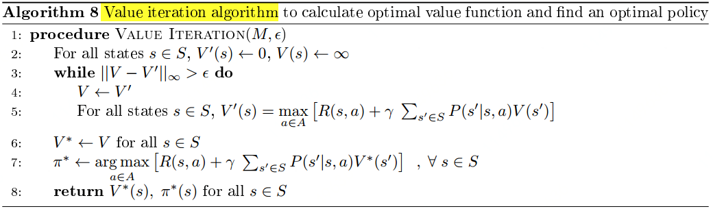
Code Implementaion:

def value_iteration(P, nS, nA, gamma=0.9, tol=1e-3):
    """
    Learn value function and policy by using value iteration method for a given
    gamma and environment.

    Parameters:
    ----------
    P, nS, nA, gamma:
        defined at beginning of file
    tol: float
        Terminate value iteration when
            max |value_function(s) - prev_value_function(s)| < tol
    Returns:
    ----------
    value_function: np.ndarray[nS]
    policy: np.ndarray[nS]
    """
    value_function = np.zeros(nS)
    policy = np.zeros(nS, dtype=int)
    while True:
        delta = 0.
        for s in range(nS):
            v_fn = value_function[s]
            action_value = []
            for a in range(nA):
                [(prob, next_state, reward, done)] = P[s][a]
                action_value.append( prob * (reward + gamma * value_function[next_state]))
            value_function[s] = np.max(action_value)
            policy[s] = np.argmax(action_value)
            delta = np.maximum(delta, np.abs(v_fn - value_function[s]))
        if delta < tol:
            break
    return value_function, policy

def value_iteration(P, nS, nA, gamma=0.9, tol=1e-3):

"""

Learn value function and policy by using value iteration method for a given

gamma and environment.

Parameters:

----------

P, nS, nA, gamma:

defined at beginning of file

tol: float

Terminate value iteration when

max |value_function(s) - prev_value_function(s)| < tol

Returns:

----------

value_function: np.ndarray[nS]

policy: np.ndarray[nS]

"""

value_function = np.zeros(nS)

policy = np.zeros(nS, dtype=int)

while True:

delta = 0.

for s in range(nS):

v_fn = value_function[s]

action_value = []

for a in range(nA):

[(prob, next_state, reward, done)] = P[s][a]

action_value.append( prob * (reward + gamma * value_function[next_state]))

value_function[s] = np.max(action_value)

policy[s] = np.argmax(action_value)

delta = np.maximum(delta, np.abs(v_fn - value_function[s]))

if delta < tol:

break

return value_function, policy

2.5 Policy Search

Pseudocode:

3. Examples

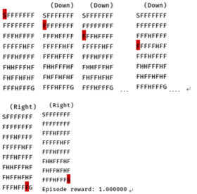
3.1 Frozen Lake

Problem Discription:
S: the starting position
F: the frozen lake where you can walk
H: holes, which have to be careful about to avoid
G: the goal
Code Implementation.

### MDP Value Iteration and Policy Iteration

import numpy as np
import gym
import time
from lake_envs import *

np.set_printoptions(precision=3)

"""
For policy_evaluation, policy_improvement, policy_iteration and value_iteration,
the parameters P, nS, nA, gamma are defined as follows:

    P: nested dictionary
        From gym.core.Environment
        For each pair of states in [1, nS] and actions in [1, nA], P[state][action] is a
        tuple of the form (probability, nextstate, reward, terminal) where
            - probability: float
                the probability of transitioning from "state" to "nextstate" with "action"
            - nextstate: int
                denotes the state we transition to (in range [0, nS - 1])
            - reward: int
                either 0 or 1, the reward for transitioning from "state" to
                "nextstate" with "action"
            - terminal: bool
              True when "nextstate" is a terminal state (hole or goal), False otherwise
    nS: int
        number of states in the environment
    nA: int
        number of actions in the environment
    gamma: float
        Discount factor. Number in range [0, 1)
"""

def policy_evaluation(P, nS, nA, policy, gamma=0.9, tol=1e-3):
    """Evaluate the value function from a given policy.

    Parameters
    ----------
    P, nS, nA, gamma:
        defined at beginning of file
    policy: np.array[nS]
        The policy to evaluate. Maps states to actions.
    tol: float
        Terminate policy evaluation when
            max |value_function(s) - prev_value_function(s)| < tol
    Returns
    -------
    value_function: np.ndarray[nS]
        The value function of the given policy, where value_function[s] is
        the value of state s
    """

    value_function = np.zeros(nS)

    while True:
        # new value function
        new_value_function = np.zeros(nS)

        # loop over state
        for s in range(nS):
            # To accumelate bellman expectation eqn with respect to actions
            for a in range(nA):
                # get transitions
                [(prob, next_state, reward, done)] = P[s][a]
                # apply bellman expectatoin eqn
                # Here assuming action_prob = 0.25, can also get from policy
                new_value_function[s] += 0.25 * prob * (reward + gamma * value_function[next_state])

        delta = np.max(np.abs(new_value_function - value_function))
        # the new value function
        value_function = new_value_function
        if delta < tol:
            break
    return value_function

def policy_improvement(P, nS, nA, value_from_policy, policy, gamma=0.9):
    """Given the value function from policy improve the policy.

    Parameters
    ----------
    P, nS, nA, gamma:
        defined at beginning of file
    value_from_policy: np.ndarray
        The value calculated from the policy
    policy: np.array
        The previous policy.

    Returns
    -------
    new_policy: np.ndarray[nS]
        An array of integers. Each integer is the optimal action to take
        in that state according to the environment dynamics and the
        given value function.
    """
    new_policy = np.zeros(nS, dtype='int')
    for s in range(nS):
        action_reward = []
        for a in range(nA):
            prob, next_state, reward, done = P[s][a][0]
            action_reward.append(reward + gamma * prob * value_from_policy[next_state])
        new_policy[s] = np.argmax(action_reward)
    return new_policy

def policy_iteration(P, nS, nA, gamma=0.9, tol=10e-3):
    """Runs policy iteration.

    You should call the policy_evaluation() and policy_improvement() methods to
    implement this method.

    Parameters
    ----------
    P, nS, nA, gamma:
        defined at beginning of file
    tol: float
        tol parameter used in policy_evaluation()
    Returns:
    ----------
    value_function: np.ndarray[nS]
    policy: np.ndarray[nS]
    """

    # value_function = np.zeros(nS)
    policy = np.zeros(nS, dtype=int)

    while True:
        value_function = policy_evaluation(P, nS, nA, policy, gamma, tol)
        new_policy = policy_improvement(P, nS, nA, value_function, policy, gamma)
        policy_change = (new_policy != policy).sum()
        policy = new_policy
        if policy_change == 0:
            break
    return value_function, policy

def value_iteration(P, nS, nA, gamma=0.9, tol=1e-3):
    """
    Learn value function and policy by using value iteration method for a given
    gamma and environment.

    Parameters:
    ----------
    P, nS, nA, gamma:
        defined at beginning of file
    tol: float
        Terminate value iteration when
            max |value_function(s) - prev_value_function(s)| < tol
    Returns:
    ----------
    value_function: np.ndarray[nS]
    policy: np.ndarray[nS]
    """
    value_function = np.zeros(nS)
    policy = np.zeros(nS, dtype=int)
    while True:
        delta = 0.
        for s in range(nS):
            v_fn = value_function[s]
            action_value = []
            for a in range(nA):
                [(prob, next_state, reward, done)] = P[s][a]
                action_value.append( prob * (reward + gamma * value_function[next_state]))
            value_function[s] = np.max(action_value)
            policy[s] = np.argmax(action_value)
            delta = np.maximum(delta, np.abs(v_fn - value_function[s]))
        if delta < tol:
            break
    return value_function, policy

def render_single(env, policy, max_steps=100):
  """
    This function does not need to be modified
    Renders policy once on environment. Watch your agent play!

    Parameters
    ----------
    env: gym.core.Environment
      Environment to play on. Must have nS, nA, and P as
      attributes.
    Policy: np.array of shape [env.nS]
      The action to take at a given state
  """

  episode_reward = 0
  ob = env.reset()
  for t in range(max_steps):
    env.render()
    time.sleep(0.25)
    a = policy[ob]
    ob, rew, done, _ = env.step(a)
    episode_reward += rew
    if done:
      break
  env.render()
  if not done:
    print("The agent didn't reach a terminal state in {} steps.".format(max_steps))
  else:
    print("Episode reward: %f" % episode_reward)


# Edit below to run policy and value iteration on different environments and
# visualize the resulting policies in action!
# You may change the parameters in the functions below
if __name__ == "__main__":
    # comment/uncomment these lines to switch between deterministic/stochastic environments
    # env = gym.make("Deterministic-4x4-FrozenLake-v0")
    # env = gym.make("Stochastic-4x4-FrozenLake-v0")
    env = gym.make("Deterministic-8x8-FrozenLake-v0")

    print("\n" + "-"*25 + "\nBeginning Policy Iteration\n" + "-"*25)

    V_pi, p_pi = policy_iteration(env.P, env.nS, env.nA, gamma=0.9, tol=1e-3)
    render_single(env, p_pi, 100)

    print("\n" + "-"*25 + "\nBeginning Value Iteration\n" + "-"*25)

    V_vi, p_vi = value_iteration(env.P, env.nS, env.nA, gamma=0.9, tol=1e-3)
    render_single(env, p_vi, 100)

100

101

102

103

104

105

106

107

108

109

110

111

112

113

114

115

116

117

118

119

120

121

122

123

124

125

126

127

128

129

130

131

132

133

134

135

136

137

138

139

140

141

142

143

144

145

146

147

148

149

150

151

152

153

154

155

156

157

158

159

160

161

162

163

164

165

166

167

168

169

170

171

172

173

174

175

176

177

178

179

180

181

182

183

184

185

186

187

188

189

190

191

192

193

194

195

196

197

198

199

200

201

202

203

204

205

206

207

208

209

210

211

212

213

214

215

216

217

### MDP Value Iteration and Policy Iteration

import numpy as np

import gym

import time

from lake_envs import *

np.set_printoptions(precision=3)

"""

For policy_evaluation, policy_improvement, policy_iteration and value_iteration,

the parameters P, nS, nA, gamma are defined as follows:

P: nested dictionary

From gym.core.Environment

For each pair of states in [1, nS] and actions in [1, nA], P[state][action] is a

tuple of the form (probability, nextstate, reward, terminal) where

- probability: float

the probability of transitioning from "state" to "nextstate" with "action"

- nextstate: int

denotes the state we transition to (in range [0, nS - 1])

- reward: int

either 0 or 1, the reward for transitioning from "state" to

"nextstate" with "action"

- terminal: bool

True when "nextstate" is a terminal state (hole or goal), False otherwise

nS: int

number of states in the environment

nA: int

number of actions in the environment

gamma: float

Discount factor. Number in range [0, 1)

"""

def policy_evaluation(P, nS, nA, policy, gamma=0.9, tol=1e-3):

"""Evaluate the value function from a given policy.

Parameters

----------

P, nS, nA, gamma:

defined at beginning of file

policy: np.array[nS]

The policy to evaluate. Maps states to actions.

tol: float

Terminate policy evaluation when

max |value_function(s) - prev_value_function(s)| < tol

Returns

-------

value_function: np.ndarray[nS]

The value function of the given policy, where value_function[s] is

the value of state s

"""

value_function = np.zeros(nS)

while True:

# new value function

new_value_function = np.zeros(nS)

# loop over state

for s in range(nS):

# To accumelate bellman expectation eqn with respect to actions

for a in range(nA):

# get transitions

[(prob, next_state, reward, done)] = P[s][a]

# apply bellman expectatoin eqn

# Here assuming action_prob = 0.25, can also get from policy

new_value_function[s] += 0.25 * prob * (reward + gamma * value_function[next_state])

delta = np.max(np.abs(new_value_function - value_function))

# the new value function

value_function = new_value_function

if delta < tol:

break

return value_function

def policy_improvement(P, nS, nA, value_from_policy, policy, gamma=0.9):

"""Given the value function from policy improve the policy.

Parameters

----------

P, nS, nA, gamma:

defined at beginning of file

value_from_policy: np.ndarray

The value calculated from the policy

policy: np.array

The previous policy.

Returns

-------

new_policy: np.ndarray[nS]

An array of integers. Each integer is the optimal action to take

in that state according to the environment dynamics and the

given value function.

"""

new_policy = np.zeros(nS, dtype='int')

for s in range(nS):

action_reward = []

for a in range(nA):

prob, next_state, reward, done = P[s][a][0]

action_reward.append(reward + gamma * prob * value_from_policy[next_state])

new_policy[s] = np.argmax(action_reward)

return new_policy

def policy_iteration(P, nS, nA, gamma=0.9, tol=10e-3):

"""Runs policy iteration.

You should call the policy_evaluation() and policy_improvement() methods to

implement this method.

Parameters

----------

P, nS, nA, gamma:

defined at beginning of file

tol: float

tol parameter used in policy_evaluation()

Returns:

----------

value_function: np.ndarray[nS]

policy: np.ndarray[nS]

"""

# value_function = np.zeros(nS)

policy = np.zeros(nS, dtype=int)

while True:

value_function = policy_evaluation(P, nS, nA, policy, gamma, tol)

new_policy = policy_improvement(P, nS, nA, value_function, policy, gamma)

policy_change = (new_policy != policy).sum()

policy = new_policy

if policy_change == 0:

break

return value_function, policy

def value_iteration(P, nS, nA, gamma=0.9, tol=1e-3):

"""

Learn value function and policy by using value iteration method for a given

gamma and environment.

Parameters:

----------

P, nS, nA, gamma:

defined at beginning of file

tol: float

Terminate value iteration when

max |value_function(s) - prev_value_function(s)| < tol

Returns:

----------

value_function: np.ndarray[nS]

policy: np.ndarray[nS]

"""

value_function = np.zeros(nS)

policy = np.zeros(nS, dtype=int)

while True:

delta = 0.

for s in range(nS):

v_fn = value_function[s]

action_value = []

for a in range(nA):

[(prob, next_state, reward, done)] = P[s][a]

action_value.append( prob * (reward + gamma * value_function[next_state]))

value_function[s] = np.max(action_value)

policy[s] = np.argmax(action_value)

delta = np.maximum(delta, np.abs(v_fn - value_function[s]))

if delta < tol:

break

return value_function, policy

def render_single(env, policy, max_steps=100):

"""

This function does not need to be modified

Renders policy once on environment. Watch your agent play!

Parameters

----------

env: gym.core.Environment

Environment to play on. Must have nS, nA, and P as

attributes.

Policy: np.array of shape [env.nS]

The action to take at a given state

"""

episode_reward = 0

ob = env.reset()

for t in range(max_steps):

env.render()

time.sleep(0.25)

a = policy[ob]

ob, rew, done, _ = env.step(a)

episode_reward += rew

if done:

break

env.render()

if not done:

print("The agent didn't reach a terminal state in {} steps.".format(max_steps))

else:

print("Episode reward: %f" % episode_reward)

# Edit below to run policy and value iteration on different environments and

# visualize the resulting policies in action!

# You may change the parameters in the functions below

if __name__ == "__main__":

# comment/uncomment these lines to switch between deterministic/stochastic environments

# env = gym.make("Deterministic-4x4-FrozenLake-v0")

# env = gym.make("Stochastic-4x4-FrozenLake-v0")

env = gym.make("Deterministic-8x8-FrozenLake-v0")

print("\n" + "-"*25 + "\nBeginning Policy Iteration\n" + "-"*25)

V_pi, p_pi = policy_iteration(env.P, env.nS, env.nA, gamma=0.9, tol=1e-3)

render_single(env, p_pi, 100)

print("\n" + "-"*25 + "\nBeginning Value Iteration\n" + "-"*25)

V_vi, p_vi = value_iteration(env.P, env.nS, env.nA, gamma=0.9, tol=1e-3)

render_single(env, p_vi, 100)

The result for the above implementation is:

4. Summary

Both value-iteration and policy-iteration assume that the agent knows the MDP model of the world (i.e. the agent knows the state-transition and reward probability functions).Therefore, they can be used by the agent to (offline) plan its actions given knowledge about the environment before interacting with it.
In Value Iteration, we don’t make multiple steps because once the VF is optimal, then the policy converges (meaning it is also optimal). Whereas at policy iteration we do multiple steps in each iteration where every step gives us a different V(s) and the corresponding policy.

LIAO YONG Technology Space

Dynamic Programming in Reinforcement Learning

1. Dynamic Programming Overview

2. Solving DP Problems

2.3 Policy Iteration

2.4 Value Iteration

2.5 Policy Search

3. Examples

3.1 Frozen Lake

4. Summary

Leave a Reply Cancel reply