Natural Policy Gradient – LIAO YONG Technology Space

Natural Gradient shares some common ideas with the high-level policy-based methods like Trust Region Policy Optimization (TRPO), Proximal Policy Optimization (PPO) and etc. The basic idea of natural policy gradient is to use the curvature information of the of the policy’s distribution over actions in the weight update. We will explain in detail how it is formulated and applied in this post.

1. Minorize-Maximization, MM

The MM algorithm is not an algorithm, but a strategy for constructing optimization algorithms.The main idea of MM (minorization-maximization) algorithms is that, intuitively, for a maximization problem, we first find a approximated lower bound of the original objective as the surrogate objective and then maximize the approximated lower bound so as to optimize the original objective. (And vice versa for minimization problems) In minimization MM stands for Majorize–Minimize, and in maximization MM stands for Minorize–Maximize. The EM algorithm can be thought as a special case of MM.
The explanation of MM (Reference:Wikipedia)
Take the minorize-maximization version for example, let $f\left( \theta \right)$ be the objective concave function to be maximized. At the $m (m=0,1,...)$ step of the algorithm, the constructed function $g\left( {\theta \left| {{\theta _m}} \right.} \right)$ is the surrogate function at ${{\theta _m}}$ if

$\begin{array}{l}g\left( {\theta \left| {{\theta _m}} \right.} \right) \le f\left( \theta \right){\kern 1pt} {\kern 1pt} {\kern 1pt} {\kern 1pt} {\kern 1pt} {\kern 1pt} for{\kern 1pt} {\kern 1pt} {\kern 1pt} all{\kern 1pt} {\kern 1pt} {\kern 1pt} \theta \\g\left( {{\theta _m}\left| {{\theta _m}} \right.} \right) = f\left( {{\theta _m}} \right)\end{array}$

Then, we can maximize $g\left( {{\theta _m}\left| {{\theta _m}} \right.} \right)$ instead of $f\left( \theta \right)$ , in the new iteration, let

${\theta _{m + 1}} = \mathop {\arg \max }\limits_\theta g\left( {\theta \left| {{\theta _m}} \right.} \right)$

The above iteration method will guarantee that $f\left( {{\theta _m}} \right)$ will converge to a local optimum or a saddle point as $m$ goes to infinity.
Now, we get

$f\left( {{\theta _{m + 1}}} \right) \ge g\left( {{\theta _{m + 1}}\left| {{\theta _m}} \right.} \right) \ge g\left( {{\theta _m}\left| {{\theta _m}} \right.} \right) = f\left( {{\theta _m}} \right)$

The iteration process and the surrogate functions is show in below figure

Benifit of MM that substituting a simple optimization problem for a difficult problem can turn a non-differential problem into a smooth problem and linearize an optimization problem.

2. Fisher Information Matrix

Suppose we are using a model parameterized by parameter vector $\theta$ to model a distribution $p\left( {x\left| \theta \right.} \right)$ , the parameter $\theta$ can be learned by maximizing the likelikhood $p\left( {x\left| \theta \right.} \right)$ with respect to $\theta$ . To measure to the goodness of this estimation of $\theta$ , we define the gradient of log likelihood function of $p\left( {x\left| \theta \right.} \right)$ as the score function:

$s\left( \theta \right) = {\nabla _\theta }\log p\left( {x\left| \theta \right.} \right)$

One important feature of the score function is the expected value of score with respect to the model is 0.

$\begin{array}{l}\mathop \mathbb{E}\limits_{p\left( {x\left| \theta \right.} \right)} \left[ {s\left( \theta \right)} \right] = \mathop \mathbb{E}\limits_{p\left( {x\left| \theta \right.} \right)} \left[ {{\nabla _\theta }\log p\left( {x\left| \theta \right.} \right)} \right]\\{\kern 1pt} {\kern 1pt} {\kern 1pt} {\kern 1pt} {\kern 1pt} {\kern 1pt} {\kern 1pt} {\kern 1pt} {\kern 1pt} {\kern 1pt} {\kern 1pt} {\kern 1pt} {\kern 1pt} {\kern 1pt} {\kern 1pt} {\kern 1pt} {\kern 1pt} {\kern 1pt} {\kern 1pt} {\kern 1pt} {\kern 1pt} {\kern 1pt} {\kern 1pt} {\kern 1pt} {\kern 1pt} {\kern 1pt} {\kern 1pt} {\kern 1pt} {\kern 1pt} {\kern 1pt} {\kern 1pt} {\kern 1pt} {\kern 1pt} {\kern 1pt} {\kern 1pt} {\kern 1pt} {\kern 1pt} {\kern 1pt} {\kern 1pt} {\kern 1pt} {\kern 1pt} {\kern 1pt} {\kern 1pt} {\kern 1pt} {\kern 1pt} {\kern 1pt} {\kern 1pt} {\kern 1pt} {\kern 1pt} {\kern 1pt} {\kern 1pt} {\kern 1pt} {\kern 1pt} {\kern 1pt} = \int {{\nabla _\theta }\log p\left( {x\left| \theta \right.} \right)} p\left( {x\left| \theta \right.} \right)dx\\{\kern 1pt} {\kern 1pt} {\kern 1pt} {\kern 1pt} {\kern 1pt} {\kern 1pt} {\kern 1pt} {\kern 1pt} {\kern 1pt} {\kern 1pt} {\kern 1pt} {\kern 1pt} {\kern 1pt} {\kern 1pt} {\kern 1pt} {\kern 1pt} {\kern 1pt} {\kern 1pt} {\kern 1pt} {\kern 1pt} {\kern 1pt} {\kern 1pt} {\kern 1pt} {\kern 1pt} {\kern 1pt} {\kern 1pt} {\kern 1pt} {\kern 1pt} {\kern 1pt} {\kern 1pt} {\kern 1pt} {\kern 1pt} {\kern 1pt} {\kern 1pt} {\kern 1pt} {\kern 1pt} {\kern 1pt} {\kern 1pt} {\kern 1pt} {\kern 1pt} {\kern 1pt} {\kern 1pt} {\kern 1pt} {\kern 1pt} {\kern 1pt} {\kern 1pt} {\kern 1pt} {\kern 1pt} {\kern 1pt} {\kern 1pt} {\kern 1pt} {\kern 1pt} {\kern 1pt} = \int {\frac{{{\nabla _\theta }p\left( {x\left| \theta \right.} \right)}}{{p\left( {x\left| \theta \right.} \right)}}} p\left( {x\left| \theta \right.} \right)dx\\{\kern 1pt} {\kern 1pt} {\kern 1pt} {\kern 1pt} {\kern 1pt} {\kern 1pt} {\kern 1pt} {\kern 1pt} {\kern 1pt} {\kern 1pt} {\kern 1pt} {\kern 1pt} {\kern 1pt} {\kern 1pt} {\kern 1pt} {\kern 1pt} {\kern 1pt} {\kern 1pt} {\kern 1pt} {\kern 1pt} {\kern 1pt} {\kern 1pt} {\kern 1pt} {\kern 1pt} {\kern 1pt} {\kern 1pt} {\kern 1pt} {\kern 1pt} {\kern 1pt} {\kern 1pt} {\kern 1pt} {\kern 1pt} {\kern 1pt} {\kern 1pt} {\kern 1pt} {\kern 1pt} {\kern 1pt} {\kern 1pt} {\kern 1pt} {\kern 1pt} {\kern 1pt} {\kern 1pt} {\kern 1pt} {\kern 1pt} {\kern 1pt} {\kern 1pt} {\kern 1pt} {\kern 1pt} {\kern 1pt} {\kern 1pt} {\kern 1pt} {\kern 1pt} = \int {{\nabla _\theta }p\left( {x\left| \theta \right.} \right)dx} \\{\kern 1pt} {\kern 1pt} {\kern 1pt} {\kern 1pt} {\kern 1pt} {\kern 1pt} {\kern 1pt} {\kern 1pt} {\kern 1pt} {\kern 1pt} {\kern 1pt} {\kern 1pt} {\kern 1pt} {\kern 1pt} {\kern 1pt} {\kern 1pt} {\kern 1pt} {\kern 1pt} {\kern 1pt} {\kern 1pt} {\kern 1pt} {\kern 1pt} {\kern 1pt} {\kern 1pt} {\kern 1pt} {\kern 1pt} {\kern 1pt} {\kern 1pt} {\kern 1pt} {\kern 1pt} {\kern 1pt} {\kern 1pt} {\kern 1pt} {\kern 1pt} {\kern 1pt} {\kern 1pt} {\kern 1pt} {\kern 1pt} {\kern 1pt} {\kern 1pt} {\kern 1pt} {\kern 1pt} {\kern 1pt} {\kern 1pt} {\kern 1pt} {\kern 1pt} {\kern 1pt} {\kern 1pt} {\kern 1pt} {\kern 1pt} {\kern 1pt} = {\nabla _\theta }\int {p\left( {x\left| \theta \right.} \right)dx} \\{\kern 1pt} {\kern 1pt} {\kern 1pt} {\kern 1pt} {\kern 1pt} {\kern 1pt} {\kern 1pt} {\kern 1pt} {\kern 1pt} {\kern 1pt} {\kern 1pt} {\kern 1pt} {\kern 1pt} {\kern 1pt} {\kern 1pt} {\kern 1pt} {\kern 1pt} {\kern 1pt} {\kern 1pt} {\kern 1pt} {\kern 1pt} {\kern 1pt} {\kern 1pt} {\kern 1pt} {\kern 1pt} {\kern 1pt} {\kern 1pt} {\kern 1pt} {\kern 1pt} {\kern 1pt} {\kern 1pt} {\kern 1pt} {\kern 1pt} {\kern 1pt} {\kern 1pt} {\kern 1pt} {\kern 1pt} {\kern 1pt} {\kern 1pt} {\kern 1pt} {\kern 1pt} {\kern 1pt} {\kern 1pt} {\kern 1pt} {\kern 1pt} {\kern 1pt} {\kern 1pt} {\kern 1pt} {\kern 1pt} {\kern 1pt} = {\nabla _\theta }1\\{\kern 1pt} {\kern 1pt} {\kern 1pt} {\kern 1pt} {\kern 1pt} {\kern 1pt} {\kern 1pt} {\kern 1pt} {\kern 1pt} {\kern 1pt} {\kern 1pt} {\kern 1pt} {\kern 1pt} {\kern 1pt} {\kern 1pt} {\kern 1pt} {\kern 1pt} {\kern 1pt} {\kern 1pt} {\kern 1pt} {\kern 1pt} {\kern 1pt} {\kern 1pt} {\kern 1pt} {\kern 1pt} {\kern 1pt} {\kern 1pt} {\kern 1pt} {\kern 1pt} {\kern 1pt} {\kern 1pt} {\kern 1pt} {\kern 1pt} {\kern 1pt} {\kern 1pt} {\kern 1pt} {\kern 1pt} {\kern 1pt} {\kern 1pt} {\kern 1pt} {\kern 1pt} {\kern 1pt} {\kern 1pt} {\kern 1pt} {\kern 1pt} {\kern 1pt} {\kern 1pt} {\kern 1pt} {\kern 1pt} = 0\end{array}$

Fisher Information: the covariance of the score function.
Here, the covariance defined as an uncertainty measure around the expected estimate is used to measure how certain we are to the estimate:

$\mathop \mathbb{E}\limits_{p\left( {x\left| \theta \right.} \right)} \left[ {\left( {s\left( \theta \right) - 0} \right){{\left( {s\left( \theta \right) - 0} \right)}^{\rm{T}}}} \right]$

Thus, for parameters vector $\theta$ , Fisher Information is in a matrix form called Fisher Information Matrix and denoted as:

$\mathbb{F} = \mathop \mathbb{E}\limits_{p\left( {x\left| \theta \right.} \right)} \left[ {{\nabla _\theta }\log p\left( {x\left| \theta \right.} \right){\nabla _\theta }\log p{{\left( {x\left| \theta \right.} \right)}^{\rm{T}}}} \right]$

In practice, analytical solution for the above average is intractable and replaced by calculating average using sampling data $X = \left\{ {{x_1},{x_2}, \cdots ,{x_N}} \right\}$ from empirical distribution $\hat q\left( x \right)$ . Then $\mathbb{F}$ here is called Empirical Fisher:

$\mathbb{F} = \frac{1}{N}\sum\limits_{i = 1}^N {{\nabla _\theta }\log p\left( {{x_i}\left| \theta \right.} \right){\nabla _\theta }\log p{{\left( {{x_i}\left| \theta \right.} \right)}^{\rm{T}}}}$

Fisher and Hessian
Feature: the negative expected Hessian of log likelihood is equal to the Fisher Information Matrix $\mathbb{F}$
Proof:

$\begin{array}{l}{{\rm{H}}_{\log p\left( {x\left| \theta \right.} \right)}} = Jacobian\left( {\frac{{{\nabla _\theta }p\left( {x\left| \theta \right.} \right)}}{{p\left( {x\left| \theta \right.} \right)}}} \right)\\{\kern 1pt} {\kern 1pt} {\kern 1pt} {\kern 1pt} {\kern 1pt} {\kern 1pt} {\kern 1pt} {\kern 1pt} {\kern 1pt} {\kern 1pt} {\kern 1pt} {\kern 1pt} {\kern 1pt} {\kern 1pt} {\kern 1pt} {\kern 1pt} {\kern 1pt} {\kern 1pt} {\kern 1pt} {\kern 1pt} {\kern 1pt} {\kern 1pt} {\kern 1pt} {\kern 1pt} {\kern 1pt} {\kern 1pt} {\kern 1pt} {\kern 1pt} {\kern 1pt} {\kern 1pt} {\kern 1pt} {\kern 1pt} {\kern 1pt} {\kern 1pt} {\kern 1pt} {\kern 1pt} {\kern 1pt} {\kern 1pt} {\kern 1pt} = \frac{{{{\rm{H}}_{p\left( {x\left| \theta \right.} \right)}}p\left( {x\left| \theta \right.} \right) - {\nabla _\theta }p\left( {x\left| \theta \right.} \right){\nabla _\theta }p{{\left( {x\left| \theta \right.} \right)}^T}}}{{p\left( {x\left| \theta \right.} \right)p\left( {x\left| \theta \right.} \right)}}\\{\kern 1pt} {\kern 1pt} {\kern 1pt} {\kern 1pt} {\kern 1pt} {\kern 1pt} {\kern 1pt} {\kern 1pt} {\kern 1pt} {\kern 1pt} {\kern 1pt} {\kern 1pt} {\kern 1pt} {\kern 1pt} {\kern 1pt} {\kern 1pt} {\kern 1pt} {\kern 1pt} {\kern 1pt} {\kern 1pt} {\kern 1pt} {\kern 1pt} {\kern 1pt} {\kern 1pt} {\kern 1pt} {\kern 1pt} {\kern 1pt} {\kern 1pt} {\kern 1pt} {\kern 1pt} {\kern 1pt} {\kern 1pt} {\kern 1pt} {\kern 1pt} {\kern 1pt} {\kern 1pt} {\kern 1pt} {\kern 1pt} = \frac{{{{\rm{H}}_{p\left( {x\left| \theta \right.} \right)}}p\left( {x\left| \theta \right.} \right)}}{{p\left( {x\left| \theta \right.} \right)p\left( {x\left| \theta \right.} \right)}} - \frac{{{\nabla _\theta }p\left( {x\left| \theta \right.} \right){\nabla _\theta }p{{\left( {x\left| \theta \right.} \right)}^T}}}{{p\left( {x\left| \theta \right.} \right)p\left( {x\left| \theta \right.} \right)}}\\{\kern 1pt} {\kern 1pt} {\kern 1pt} {\kern 1pt} {\kern 1pt} {\kern 1pt} {\kern 1pt} {\kern 1pt} {\kern 1pt} {\kern 1pt} {\kern 1pt} {\kern 1pt} {\kern 1pt} {\kern 1pt} {\kern 1pt} {\kern 1pt} {\kern 1pt} {\kern 1pt} {\kern 1pt} {\kern 1pt} {\kern 1pt} {\kern 1pt} {\kern 1pt} {\kern 1pt} {\kern 1pt} {\kern 1pt} {\kern 1pt} {\kern 1pt} {\kern 1pt} {\kern 1pt} {\kern 1pt} {\kern 1pt} {\kern 1pt} {\kern 1pt} {\kern 1pt} {\kern 1pt} {\kern 1pt} = \frac{{{{\rm{H}}_{p\left( {x\left| \theta \right.} \right)}}}}{{p\left( {x\left| \theta \right.} \right)}} - \left( {\frac{{{\nabla _\theta }p\left( {x\left| \theta \right.} \right)}}{{p\left( {x\left| \theta \right.} \right)}}} \right){\left( {\frac{{{\nabla _\theta }p\left( {x\left| \theta \right.} \right)}}{{p\left( {x\left| \theta \right.} \right)}}} \right)^T}\end{array}$

Then, the expected of Hessian is

$\begin{array}{l}\mathop \mathbb{E}\limits_{p\left( {x\left| \theta \right.} \right)} \left[ {{{\rm{H}}_{\log p\left( {x\left| \theta \right.} \right)}}} \right] = \mathop \mathbb{E}\limits_{p\left( {x\left| \theta \right.} \right)} \left[ {\frac{{{{\rm{H}}_{p\left( {x\left| \theta \right.} \right)}}}}{{p\left( {x\left| \theta \right.} \right)}} - \left( {\frac{{{\nabla _\theta }p\left( {x\left| \theta \right.} \right)}}{{p\left( {x\left| \theta \right.} \right)}}} \right){{\left( {\frac{{{\nabla _\theta }p\left( {x\left| \theta \right.} \right)}}{{p\left( {x\left| \theta \right.} \right)}}} \right)}^T}} \right]\\{\kern 1pt} {\kern 1pt} {\kern 1pt} {\kern 1pt} {\kern 1pt} {\kern 1pt} {\kern 1pt} {\kern 1pt} {\kern 1pt} {\kern 1pt} {\kern 1pt} {\kern 1pt} {\kern 1pt} {\kern 1pt} {\kern 1pt} {\kern 1pt} {\kern 1pt} {\kern 1pt} {\kern 1pt} {\kern 1pt} {\kern 1pt} {\kern 1pt} {\kern 1pt} {\kern 1pt} {\kern 1pt} {\kern 1pt} {\kern 1pt} {\kern 1pt} {\kern 1pt} {\kern 1pt} {\kern 1pt} {\kern 1pt} {\kern 1pt} {\kern 1pt} {\kern 1pt} {\kern 1pt} {\kern 1pt} {\kern 1pt} {\kern 1pt} {\kern 1pt} {\kern 1pt} {\kern 1pt} {\kern 1pt} {\kern 1pt} {\kern 1pt} {\kern 1pt} {\kern 1pt} {\kern 1pt} {\kern 1pt} {\kern 1pt} {\kern 1pt} {\kern 1pt} {\kern 1pt} {\kern 1pt} {\kern 1pt} {\kern 1pt} {\kern 1pt} {\kern 1pt} {\kern 1pt} {\kern 1pt} {\kern 1pt} {\kern 1pt} {\kern 1pt} {\kern 1pt} {\kern 1pt} {\kern 1pt} {\kern 1pt} {\kern 1pt} {\kern 1pt} {\kern 1pt} = \mathop \mathbb{E}\limits_{p\left( {x\left| \theta \right.} \right)} \left[ {\frac{{{{\rm{H}}_{p\left( {x\left| \theta \right.} \right)}}}}{{p\left( {x\left| \theta \right.} \right)}}} \right] - \mathop \mathbb{E}\limits_{p\left( {x\left| \theta \right.} \right)} \left[ {\left( {\frac{{{\nabla _\theta }p\left( {x\left| \theta \right.} \right)}}{{p\left( {x\left| \theta \right.} \right)}}} \right){{\left( {\frac{{{\nabla _\theta }p\left( {x\left| \theta \right.} \right)}}{{p\left( {x\left| \theta \right.} \right)}}} \right)}^T}} \right]\\{\kern 1pt} {\kern 1pt} {\kern 1pt} {\kern 1pt} {\kern 1pt} {\kern 1pt} {\kern 1pt} {\kern 1pt} {\kern 1pt} {\kern 1pt} {\kern 1pt} {\kern 1pt} {\kern 1pt} {\kern 1pt} {\kern 1pt} {\kern 1pt} {\kern 1pt} {\kern 1pt} {\kern 1pt} {\kern 1pt} {\kern 1pt} {\kern 1pt} {\kern 1pt} {\kern 1pt} {\kern 1pt} {\kern 1pt} {\kern 1pt} {\kern 1pt} {\kern 1pt} {\kern 1pt} {\kern 1pt} {\kern 1pt} {\kern 1pt} {\kern 1pt} {\kern 1pt} {\kern 1pt} {\kern 1pt} {\kern 1pt} {\kern 1pt} {\kern 1pt} {\kern 1pt} {\kern 1pt} {\kern 1pt} {\kern 1pt} {\kern 1pt} {\kern 1pt} {\kern 1pt} {\kern 1pt} {\kern 1pt} {\kern 1pt} {\kern 1pt} {\kern 1pt} {\kern 1pt} {\kern 1pt} {\kern 1pt} {\kern 1pt} {\kern 1pt} {\kern 1pt} {\kern 1pt} {\kern 1pt} {\kern 1pt} {\kern 1pt} {\kern 1pt} {\kern 1pt} {\kern 1pt} {\kern 1pt} {\kern 1pt} {\kern 1pt} {\kern 1pt} = \int {\frac{{{{\rm{H}}_{p\left( {x\left| \theta \right.} \right)}}}}{{p\left( {x\left| \theta \right.} \right)}}} p\left( {x\left| \theta \right.} \right)dx - \mathop \mathbb{E}\limits_{p\left( {x\left| \theta \right.} \right)} \left[ {{\nabla _\theta }\log p\left( {x\left| \theta \right.} \right){\nabla _\theta }\log p{{\left( {x\left| \theta \right.} \right)}^{\rm{T}}}} \right]\\{\kern 1pt} {\kern 1pt} {\kern 1pt} {\kern 1pt} {\kern 1pt} {\kern 1pt} {\kern 1pt} {\kern 1pt} {\kern 1pt} {\kern 1pt} {\kern 1pt} {\kern 1pt} {\kern 1pt} {\kern 1pt} {\kern 1pt} {\kern 1pt} {\kern 1pt} {\kern 1pt} {\kern 1pt} {\kern 1pt} {\kern 1pt} {\kern 1pt} {\kern 1pt} {\kern 1pt} {\kern 1pt} {\kern 1pt} {\kern 1pt} {\kern 1pt} {\kern 1pt} {\kern 1pt} {\kern 1pt} {\kern 1pt} {\kern 1pt} {\kern 1pt} {\kern 1pt} {\kern 1pt} {\kern 1pt} {\kern 1pt} {\kern 1pt} {\kern 1pt} {\kern 1pt} {\kern 1pt} {\kern 1pt} {\kern 1pt} {\kern 1pt} {\kern 1pt} {\kern 1pt} {\kern 1pt} {\kern 1pt} {\kern 1pt} {\kern 1pt} {\kern 1pt} {\kern 1pt} {\kern 1pt} {\kern 1pt} {\kern 1pt} {\kern 1pt} {\kern 1pt} {\kern 1pt} {\kern 1pt} {\kern 1pt} {\kern 1pt} {\kern 1pt} {\kern 1pt} {\kern 1pt} {\kern 1pt} {\kern 1pt} {\kern 1pt} = {{\rm{H}}_{\int {p\left( {x\left| \theta \right.} \right)dx} }} - \mathbb{F}\\{\kern 1pt} {\kern 1pt} {\kern 1pt} {\kern 1pt} {\kern 1pt} {\kern 1pt} {\kern 1pt} {\kern 1pt} {\kern 1pt} {\kern 1pt} {\kern 1pt} {\kern 1pt} {\kern 1pt} {\kern 1pt} {\kern 1pt} {\kern 1pt} {\kern 1pt} {\kern 1pt} {\kern 1pt} {\kern 1pt} {\kern 1pt} {\kern 1pt} {\kern 1pt} {\kern 1pt} {\kern 1pt} {\kern 1pt} {\kern 1pt} {\kern 1pt} {\kern 1pt} {\kern 1pt} {\kern 1pt} {\kern 1pt} {\kern 1pt} {\kern 1pt} {\kern 1pt} {\kern 1pt} {\kern 1pt} {\kern 1pt} {\kern 1pt} {\kern 1pt} {\kern 1pt} {\kern 1pt} {\kern 1pt} {\kern 1pt} {\kern 1pt} {\kern 1pt} {\kern 1pt} {\kern 1pt} {\kern 1pt} {\kern 1pt} {\kern 1pt} {\kern 1pt} {\kern 1pt} {\kern 1pt} {\kern 1pt} {\kern 1pt} {\kern 1pt} {\kern 1pt} {\kern 1pt} {\kern 1pt} {\kern 1pt} {\kern 1pt} {\kern 1pt} {\kern 1pt} {\kern 1pt} {\kern 1pt} {\kern 1pt} = {{\rm{H}}_1} - \mathbb{F}\\{\kern 1pt} {\kern 1pt} {\kern 1pt} {\kern 1pt} {\kern 1pt} {\kern 1pt} {\kern 1pt} {\kern 1pt} {\kern 1pt} {\kern 1pt} {\kern 1pt} {\kern 1pt} {\kern 1pt} {\kern 1pt} {\kern 1pt} {\kern 1pt} {\kern 1pt} {\kern 1pt} {\kern 1pt} {\kern 1pt} {\kern 1pt} {\kern 1pt} {\kern 1pt} {\kern 1pt} {\kern 1pt} {\kern 1pt} {\kern 1pt} {\kern 1pt} {\kern 1pt} {\kern 1pt} {\kern 1pt} {\kern 1pt} {\kern 1pt} {\kern 1pt} {\kern 1pt} {\kern 1pt} {\kern 1pt} {\kern 1pt} {\kern 1pt} {\kern 1pt} {\kern 1pt} {\kern 1pt} {\kern 1pt} {\kern 1pt} {\kern 1pt} {\kern 1pt} {\kern 1pt} {\kern 1pt} {\kern 1pt} {\kern 1pt} {\kern 1pt} {\kern 1pt} {\kern 1pt} {\kern 1pt} {\kern 1pt} {\kern 1pt} {\kern 1pt} {\kern 1pt} {\kern 1pt} {\kern 1pt} {\kern 1pt} {\kern 1pt} {\kern 1pt} {\kern 1pt} {\kern 1pt} {\kern 1pt} = - \mathbb{F}\end{array}$

namely,

$\mathbb{F} = - \mathop \mathbb{E}\limits_{p\left( {x\left| \theta \right.} \right)} \left[ {{{\rm{H}}_{\log p\left( {x\left| \theta \right.} \right)}}} \right]$

3. Fisher Information Matrix and KL-divergence

KL divergence maps to our notion of what a probability distance should look like: it measures directly in terms of how probability density functions are defined, that is, differences in density value at a bunch of points over which the distribution is defined.
The relationship between Fisher Information Matrix and KL-divergence is that FIM defines the local curvature in distribution space for which KL-divergence is the metric. That is, FIM F is the Hessian of KL-divergence between two distributions $p\left( {x\left| \theta \right.} \right)$ and $p\left( {x\left| {\theta '} \right.} \right)$ , with respect to $\theta'$ , evaluated at $\theta ' = \theta$ .
This can be proved as follow:

$\begin{array}{l}{\rm{KL}}\left[ {p\left( {x\left| \theta \right.} \right)\left\| {p\left( {x\left| {\theta '} \right.} \right)} \right.} \right] = \mathop \mathbb{E}\limits_{p\left( {x\left| \theta \right.} \right)} \left[ {\log p\left( {x\left| \theta \right.} \right)} \right] - \mathop \mathbb{E}\limits_{p\left( {x\left| \theta \right.} \right)} \left[ {\log p\left( {x\left| {\theta '} \right.} \right)} \right]\\{\nabla _{\theta '}}{\rm{KL}}\left[ {p\left( {x\left| \theta \right.} \right)\left\| {p\left( {x\left| {\theta '} \right.} \right)} \right.} \right] = {\nabla _{\theta '}}\mathop \mathbb{E}\limits_{p\left( {x\left| \theta \right.} \right)} \left[ {\log p\left( {x\left| \theta \right.} \right)} \right] - {\nabla _{\theta '}}\mathop \mathbb{E}\limits_{p\left( {x\left| \theta \right.} \right)} \left[ {\log p\left( {x\left| {\theta '} \right.} \right)} \right]\\{\kern 1pt} {\kern 1pt} {\kern 1pt} {\kern 1pt} {\kern 1pt} {\kern 1pt} {\kern 1pt} {\kern 1pt} {\kern 1pt} {\kern 1pt} {\kern 1pt} {\kern 1pt} {\kern 1pt} {\kern 1pt} {\kern 1pt} {\kern 1pt} {\kern 1pt} {\kern 1pt} {\kern 1pt} {\kern 1pt} {\kern 1pt} {\kern 1pt} {\kern 1pt} {\kern 1pt} {\kern 1pt} {\kern 1pt} {\kern 1pt} {\kern 1pt} {\kern 1pt} {\kern 1pt} {\kern 1pt} {\kern 1pt} {\kern 1pt} {\kern 1pt} {\kern 1pt} {\kern 1pt} {\kern 1pt} {\kern 1pt} {\kern 1pt} {\kern 1pt} {\kern 1pt} {\kern 1pt} {\kern 1pt} {\kern 1pt} {\kern 1pt} {\kern 1pt} {\kern 1pt} {\kern 1pt} {\kern 1pt} {\kern 1pt} {\kern 1pt} {\kern 1pt} {\kern 1pt} {\kern 1pt} {\kern 1pt} {\kern 1pt} {\kern 1pt} {\kern 1pt} {\kern 1pt} {\kern 1pt} {\kern 1pt} {\kern 1pt} {\kern 1pt} {\kern 1pt} {\kern 1pt} {\kern 1pt} {\kern 1pt} {\kern 1pt} {\kern 1pt} {\kern 1pt} {\kern 1pt} {\kern 1pt} {\kern 1pt} {\kern 1pt} {\kern 1pt} {\kern 1pt} {\kern 1pt} {\kern 1pt} {\kern 1pt} {\kern 1pt} {\kern 1pt} {\kern 1pt} {\kern 1pt} {\kern 1pt} {\kern 1pt} {\kern 1pt} {\kern 1pt} {\kern 1pt} {\kern 1pt} {\kern 1pt} {\kern 1pt} {\kern 1pt} {\kern 1pt} {\kern 1pt} {\kern 1pt} {\kern 1pt} {\kern 1pt} {\kern 1pt} {\kern 1pt} {\kern 1pt} {\kern 1pt} {\kern 1pt} {\kern 1pt} {\kern 1pt} {\kern 1pt} {\kern 1pt} {\kern 1pt} {\kern 1pt} {\kern 1pt} {\kern 1pt} {\kern 1pt} {\kern 1pt} {\kern 1pt} {\kern 1pt} {\kern 1pt} {\kern 1pt} {\kern 1pt} {\kern 1pt} {\kern 1pt} {\kern 1pt} {\kern 1pt} {\kern 1pt} = - \mathop \mathbb{E}\limits_{p\left( {x\left| \theta \right.} \right)} \left[ {{\nabla _{\theta '}}\log p\left( {x\left| {\theta '} \right.} \right)} \right]\\{\kern 1pt} {\kern 1pt} {\kern 1pt} {\kern 1pt} {\kern 1pt} {\kern 1pt} {\kern 1pt} {\kern 1pt} {\kern 1pt} {\kern 1pt} {\kern 1pt} {\kern 1pt} {\kern 1pt} {\kern 1pt} {\kern 1pt} {\kern 1pt} {\kern 1pt} {\kern 1pt} {\kern 1pt} {\kern 1pt} {\kern 1pt} {\kern 1pt} {\kern 1pt} {\kern 1pt} {\kern 1pt} {\kern 1pt} {\kern 1pt} {\kern 1pt} {\kern 1pt} {\kern 1pt} {\kern 1pt} {\kern 1pt} {\kern 1pt} {\kern 1pt} {\kern 1pt} {\kern 1pt} {\kern 1pt} {\kern 1pt} {\kern 1pt} {\kern 1pt} {\kern 1pt} {\kern 1pt} {\kern 1pt} {\kern 1pt} {\kern 1pt} {\kern 1pt} {\kern 1pt} {\kern 1pt} {\kern 1pt} {\kern 1pt} {\kern 1pt} {\kern 1pt} {\kern 1pt} {\kern 1pt} {\kern 1pt} {\kern 1pt} {\kern 1pt} {\kern 1pt} {\kern 1pt} {\kern 1pt} {\kern 1pt} {\kern 1pt} {\kern 1pt} {\kern 1pt} {\kern 1pt} {\kern 1pt} {\kern 1pt} {\kern 1pt} {\kern 1pt} {\kern 1pt} {\kern 1pt} {\kern 1pt} {\kern 1pt} {\kern 1pt} {\kern 1pt} {\kern 1pt} {\kern 1pt} {\kern 1pt} {\kern 1pt} {\kern 1pt} {\kern 1pt} {\kern 1pt} {\kern 1pt} {\kern 1pt} {\kern 1pt} {\kern 1pt} {\kern 1pt} {\kern 1pt} {\kern 1pt} {\kern 1pt} {\kern 1pt} {\kern 1pt} {\kern 1pt} {\kern 1pt} {\kern 1pt} {\kern 1pt} {\kern 1pt} {\kern 1pt} {\kern 1pt} {\kern 1pt} {\kern 1pt} {\kern 1pt} {\kern 1pt} {\kern 1pt} {\kern 1pt} {\kern 1pt} {\kern 1pt} {\kern 1pt} {\kern 1pt} {\kern 1pt} {\kern 1pt} {\kern 1pt} {\kern 1pt} {\kern 1pt} {\kern 1pt} {\kern 1pt} {\kern 1pt} {\kern 1pt} {\kern 1pt} {\kern 1pt} {\kern 1pt} = - \int {p\left( {x\left| \theta \right.} \right)} {\nabla _{\theta '}}\log p\left( {x\left| {\theta '} \right.} \right)dx\\\nabla _{\theta '}^2{\rm{KL}}\left[ {p\left( {x\left| \theta \right.} \right)\left\| {p\left( {x\left| {\theta '} \right.} \right)} \right.} \right] = - \int {p\left( {x\left| \theta \right.} \right)} \nabla _{\theta '}^2\log p\left( {x\left| {\theta '} \right.} \right)dx\\{\rm{H}_{{\rm{KL}}\left[ {p\left( {x\left| \theta \right.} \right)\left\| {p\left( {x\left| {\theta '} \right.} \right)} \right.} \right]}} = - \int {p\left( {x\left| \theta \right.} \right)} \nabla _{\theta '}^2\log p\left( {x\left| {\theta '} \right.} \right)\left| {_{\theta ' = \theta }} \right.dx\\{\kern 1pt} {\kern 1pt} {\kern 1pt} {\kern 1pt} {\kern 1pt} {\kern 1pt} {\kern 1pt} {\kern 1pt} {\kern 1pt} {\kern 1pt} {\kern 1pt} {\kern 1pt} {\kern 1pt} {\kern 1pt} {\kern 1pt} {\kern 1pt} {\kern 1pt} {\kern 1pt} {\kern 1pt} {\kern 1pt} {\kern 1pt} {\kern 1pt} {\kern 1pt} {\kern 1pt} {\kern 1pt} {\kern 1pt} {\kern 1pt} {\kern 1pt} {\kern 1pt} {\kern 1pt} {\kern 1pt} {\kern 1pt} {\kern 1pt} {\kern 1pt} {\kern 1pt} {\kern 1pt} {\kern 1pt} {\kern 1pt} {\kern 1pt} {\kern 1pt} {\kern 1pt} {\kern 1pt} {\kern 1pt} {\kern 1pt} {\kern 1pt} {\kern 1pt} {\kern 1pt} {\kern 1pt} {\kern 1pt} {\kern 1pt} {\kern 1pt} {\kern 1pt} {\kern 1pt} {\kern 1pt} {\kern 1pt} {\kern 1pt} {\kern 1pt} {\kern 1pt} {\kern 1pt} {\kern 1pt} {\kern 1pt} {\kern 1pt} {\kern 1pt} {\kern 1pt} {\kern 1pt} {\kern 1pt} {\kern 1pt} {\kern 1pt} = - \int {p\left( {x\left| \theta \right.} \right)} {\rm{H}_{\log p\left( {x\left| \theta \right.} \right)}}dx\\{\kern 1pt} {\kern 1pt} {\kern 1pt} {\kern 1pt} {\kern 1pt} {\kern 1pt} {\kern 1pt} {\kern 1pt} {\kern 1pt} {\kern 1pt} {\kern 1pt} {\kern 1pt} {\kern 1pt} {\kern 1pt} {\kern 1pt} {\kern 1pt} {\kern 1pt} {\kern 1pt} {\kern 1pt} {\kern 1pt} {\kern 1pt} {\kern 1pt} {\kern 1pt} {\kern 1pt} {\kern 1pt} {\kern 1pt} {\kern 1pt} {\kern 1pt} {\kern 1pt} {\kern 1pt} {\kern 1pt} {\kern 1pt} {\kern 1pt} {\kern 1pt} {\kern 1pt} {\kern 1pt} {\kern 1pt} {\kern 1pt} {\kern 1pt} {\kern 1pt} {\kern 1pt} {\kern 1pt} {\kern 1pt} {\kern 1pt} {\kern 1pt} {\kern 1pt} {\kern 1pt} {\kern 1pt} {\kern 1pt} {\kern 1pt} {\kern 1pt} {\kern 1pt} {\kern 1pt} {\kern 1pt} {\kern 1pt} {\kern 1pt} {\kern 1pt} {\kern 1pt} {\kern 1pt} {\kern 1pt} {\kern 1pt} {\kern 1pt} {\kern 1pt} {\kern 1pt} {\kern 1pt} {\kern 1pt} {\kern 1pt} = - \mathop \mathbb{E}\limits_{p\left( {x\left| \theta \right.} \right)} \left[ {{\rm{H}_{\log p\left( {x\left| \theta \right.} \right)}}} \right]\\{\kern 1pt} {\kern 1pt} {\kern 1pt} {\kern 1pt} {\kern 1pt} {\kern 1pt} {\kern 1pt} {\kern 1pt} {\kern 1pt} {\kern 1pt} {\kern 1pt} {\kern 1pt} {\kern 1pt} {\kern 1pt} {\kern 1pt} {\kern 1pt} {\kern 1pt} {\kern 1pt} {\kern 1pt} {\kern 1pt} {\kern 1pt} {\kern 1pt} {\kern 1pt} {\kern 1pt} {\kern 1pt} {\kern 1pt} {\kern 1pt} {\kern 1pt} {\kern 1pt} {\kern 1pt} {\kern 1pt} {\kern 1pt} {\kern 1pt} {\kern 1pt} {\kern 1pt} {\kern 1pt} {\kern 1pt} {\kern 1pt} {\kern 1pt} {\kern 1pt} {\kern 1pt} {\kern 1pt} {\kern 1pt} {\kern 1pt} {\kern 1pt} {\kern 1pt} {\kern 1pt} {\kern 1pt} {\kern 1pt} {\kern 1pt} {\kern 1pt} {\kern 1pt} {\kern 1pt} {\kern 1pt} {\kern 1pt} {\kern 1pt} {\kern 1pt} {\kern 1pt} {\kern 1pt} {\kern 1pt} {\kern 1pt} {\kern 1pt} {\kern 1pt} {\kern 1pt} {\kern 1pt} {\kern 1pt} = \mathbb{F}\end{array}$

Since we know how to evaluate the Hessian of KL-divergence, we now see the the steepest descent in distribution space.
Using Taylor expansion, when $d \to 0$ , denote ${p\left( {x\left| \theta \right.} \right)}$ as ${p_\theta }$ for short,

$\begin{array}{l}{\rm{KL}}\left[ {p\left( {x\left| \theta \right.} \right)\left\| {p\left( {x\left| {\theta + d} \right.} \right)} \right.} \right] \approx {\rm{KL}}\left[ {p\left( {x\left| \theta \right.} \right)\left\| {p\left( {x\left| \theta \right.} \right)} \right.} \right] + {\left( {{\nabla _{\theta '}}{\rm{KL}}\left[ {p\left( {x\left| \theta \right.} \right)\left\| {p\left( {x\left| {\theta '} \right.} \right)} \right.} \right]\left| {_{\theta ' = \theta }} \right.} \right)^{\rm{T}}}d + \frac{1}{2}{d^{\rm{T}}}\rm{F}d\\{\kern 1pt} {\kern 1pt} {\kern 1pt} {\kern 1pt} {\kern 1pt} {\kern 1pt} {\kern 1pt} {\kern 1pt} {\kern 1pt} {\kern 1pt} {\kern 1pt} {\kern 1pt} {\kern 1pt} {\kern 1pt} {\kern 1pt} {\kern 1pt} {\kern 1pt} {\kern 1pt} {\kern 1pt} {\kern 1pt} {\kern 1pt} {\kern 1pt} {\kern 1pt} {\kern 1pt} {\kern 1pt} {\kern 1pt} {\kern 1pt} {\kern 1pt} {\kern 1pt} {\kern 1pt} {\kern 1pt} {\kern 1pt} {\kern 1pt} {\kern 1pt} {\kern 1pt} {\kern 1pt} {\kern 1pt} {\kern 1pt} {\kern 1pt} {\kern 1pt} {\kern 1pt} {\kern 1pt} {\kern 1pt} {\kern 1pt} {\kern 1pt} {\kern 1pt} {\kern 1pt} {\kern 1pt} {\kern 1pt} {\kern 1pt} {\kern 1pt} {\kern 1pt} {\kern 1pt} {\kern 1pt} {\kern 1pt} {\kern 1pt} {\kern 1pt} {\kern 1pt} {\kern 1pt} {\kern 1pt} {\kern 1pt} {\kern 1pt} {\kern 1pt} {\kern 1pt} {\kern 1pt} {\kern 1pt} {\kern 1pt} {\kern 1pt} {\kern 1pt} {\kern 1pt} {\kern 1pt} {\kern 1pt} {\kern 1pt} {\kern 1pt} {\kern 1pt} {\kern 1pt} {\kern 1pt} {\kern 1pt} {\kern 1pt} {\kern 1pt} {\kern 1pt} {\kern 1pt} {\kern 1pt} {\kern 1pt} {\kern 1pt} {\kern 1pt} {\kern 1pt} {\kern 1pt} {\kern 1pt} {\kern 1pt} {\kern 1pt} {\kern 1pt} {\kern 1pt} {\kern 1pt} {\kern 1pt} {\kern 1pt} {\kern 1pt} {\kern 1pt} {\kern 1pt} {\kern 1pt} {\kern 1pt} {\kern 1pt} {\kern 1pt} {\kern 1pt} {\kern 1pt} {\kern 1pt} {\kern 1pt} {\kern 1pt} {\kern 1pt} {\kern 1pt} {\kern 1pt} {\kern 1pt} {\kern 1pt} {\kern 1pt} {\kern 1pt} {\kern 1pt} {\kern 1pt} {\kern 1pt} {\kern 1pt} {\kern 1pt} {\kern 1pt} {\kern 1pt} = {\rm{KL}}\left[ {p\left( {x\left| \theta \right.} \right)\left\| {p\left( {x\left| \theta \right.} \right)} \right.} \right] - \mathop \mathbb{E}\limits_{p\left( {x\left| \theta \right.} \right)} {\left[ {{\nabla _\theta }\log p\left( {x\left| \theta \right.} \right)} \right]^{\rm{T}}} + \frac{1}{2}{d^{\rm{T}}}\rm{F}d\end{array}$

The KL-divergence for the same distribution is 0,

${\rm{KL}}\left[ {p\left( {x\left| \theta \right.} \right)\left\| {p\left( {x\left| \theta \right.} \right)} \right.} \right] = 0$

the gradient of the KL-divergence is also 0 according to the above section. So we get:

${\rm{KL}}\left[ {p\left( {x\left| \theta \right.} \right)\left\| {p\left( {x\left| {\theta + d} \right.} \right)} \right.} \right] \approx \frac{1}{2}{d^{\rm{T}}}Fd$

To minimize the loss function in distribution space, namely to find the update vector $d$ that decreases the KL-divergence the most, we can solve this minimization problem:

${d^*} = \mathop {\arg \min }\limits_{d{\kern 1pt} {\kern 1pt} s.t.{\kern 1pt} {\kern 1pt} {\kern 1pt} {\rm{KL}}\left[ {p\left( {x\left| \theta \right.} \right)\left\| {p\left( {x\left| {\theta + d} \right.} \right)} \right.} \right] = c} \mathcal{L}\left( {\theta + d} \right)$

$c$ is a constant to limit the moving speed.
To solve this minimization problem with constraint, we convert it to unconstrained problem and rewrite the equation as

$\begin{array}{l}{d^*} = \mathop {\arg \min }\limits_d \mathcal{L}\left( {\theta + d} \right) + \lambda \left( {{\rm{KL}}\left[ {p\left( {x\left| \theta \right.} \right)\left\| {p\left( {x\left| {\theta + d} \right.} \right)} \right.} \right] - c} \right)\\{\kern 1pt} {\kern 1pt} {\kern 1pt} {\kern 1pt} {\kern 1pt} {\kern 1pt} {\kern 1pt} {\kern 1pt} {\kern 1pt} {\kern 1pt} {\kern 1pt} {\kern 1pt} {\kern 1pt} \approx \mathop {\arg \min }\limits_d \mathcal{L}\left( \theta \right) + {\nabla _\theta }\mathcal{L}{\left( \theta \right)^{\rm{T}}}d + \frac{1}{2}\lambda {d^{\rm{T}}}{\rm{F}}d - \lambda c\end{array}$

This minimization problem can be solved by set its derivative with respect to d. to zero:

$\begin{array}{l}0 = \frac{\partial }{{\partial d}}\left[ {L\left( \theta \right) + {\nabla _\theta }L{{\left( \theta \right)}^{\rm{T}}}d + \frac{1}{2}\lambda {d^{\rm{T}}}{\rm{F}}d - \lambda c} \right]\\{\kern 1pt} {\kern 1pt} {\kern 1pt} {\kern 1pt} {\kern 1pt} {\kern 1pt} {\kern 1pt} {\kern 1pt} = {\nabla _\theta }\mathcal{L}\left( \theta \right) + \lambda {\rm{F}}d\end{array}$

Then we get

$d = - \frac{1}{\lambda }{{\rm{F}}^{ - 1}}{\nabla _\theta }\mathcal{L}\left( \theta \right)$

Obviously, according to the above formula, the optimal descent direction for $\mathcal{L}\left( \theta \right)$ or in Distribution Space is the opposite direction of gradient, but should take into account the local curvature in distribution space defined by ${{\rm{F}}^{ - 1}}$ .

4. Natural Policy Gradient

The Natural Gradient is defined as

$\begin{array}{l}{\nabla _\theta }\mathcal{L}\left( \theta \right) \buildrel\textstyle.\over= {\nabla _\theta }\mathcal{L}\left( \theta \right){\mathbb{E}_z}{\left[ {{{\left( {\log {p_\theta }\left( {\bf{z}} \right)} \right)}^T}\left( {\log {p_\theta }\left( {\bf{z}} \right)} \right)} \right]^{ - 1}}\\{\kern 1pt} {\kern 1pt} {\kern 1pt} {\kern 1pt} {\kern 1pt} {\kern 1pt} {\kern 1pt} {\kern 1pt} {\kern 1pt} {\kern 1pt} {\kern 1pt} {\kern 1pt} {\kern 1pt} {\kern 1pt} {\kern 1pt} {\kern 1pt} {\kern 1pt} {\kern 1pt} {\kern 1pt} {\kern 1pt} {\kern 1pt} {\kern 1pt} {\kern 1pt} {\kern 1pt} {\kern 1pt} {\kern 1pt} {\kern 1pt} {\kern 1pt} {\kern 1pt} {\kern 1pt} {\kern 1pt} {\kern 1pt} {\kern 1pt} {\kern 1pt} \buildrel\textstyle.\over= {\nabla _\theta }\mathcal{L}\left( \theta \right){\rm F^{ - 1}}\end{array}$

The “natural” bit comes from the second component: the expected value, taken over ${\bf{z}}$ , of the squared gradient of the log probability function. We take that whole object, which is referred to as the Fisher Information Matrix, and multiply our loss gradient by its inverse.
Natural Gradient provides information about curvature and a way to directly control movement of your model in predicted distribution space, as separate from movement of your model in loss space
More explanations of Natural Gradient (reference…).
Standard Gradient Decent:
Let’s say we have a neural network, parameterized by some vector of parameters. We want to adjust the parameters of this network, so the output of our network changes in some way. In most cases, we will have a loss function that tells our network how it’s output should change.
Using backpropagation, we calculate the derivatives of each parameter with respect to our loss function. These derivatives represent the direction in which we can update our parameters to get the biggest change in our loss function, and is known as the gradient. We can then adjust the parameters in the direction of the gradient, by a small distance, in order to train our network.
A slight problem appears in how we define “a small distance”.

#distance with two parameters (a,b)
distance = sqrt(a^2 + b^2)

1 2	#distance with two parameters (a,b) distance = sqrt(a^2 + b^2)

However, defining “distance” in terms of how much our parameters is adjusted isn’t always correct. To visualize this, let’s take a look at two pairs of Gaussian distributions.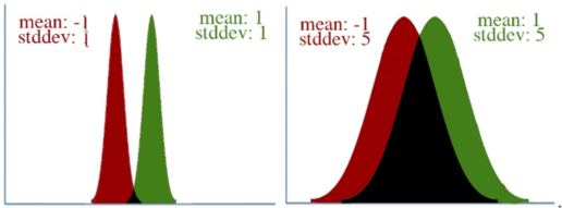
In both distributions, the mean is changed from -1 to 1, a distance of two. However, it’s clear that the first distribution changed far more than the second.This leads to a key insight: our gradient measures how much our output is affected by changing a parameter. However, this affect on the output must be seen in context: a shift of +2 in the first distribution means a lot more than a shift of +2 in the second one.
What the natural gradient does is redefine the “small distance” we update our parameters by. Not all parameters are equal. Rather than treating a change in every parameter equally, we need to scale each parameter’s change according to how much it affects our network’s entire output distribution.
How do we do that?
First off, let’s define a new form of distance, that corresponds to distance based on KL divergence, a measure of how much our new distribution differs from our old one. We do this by defining a metric matrix, which allows us to calculate the distance of a vector according to some custom measurement.
For a network with 5 parameters, our metric matrix is 5×5. To compute the distance of a change in parameters delta using metric, we use the following:

total_distance = 0
for i in xrange(5):
    for j in xrange(5):
        total_distance += delta[i] * delta[i] * metric[i][j]

total_distance = 0

for i in xrange(5):

for j in xrange(5):

total_distance += delta[i] * delta[i] * metric[i][j]

If our metric matrix is the identity matrix, the distance is the same as if we just used Euclidean distance.However, most of the time our metric won’t be the identity matrix. Having a metric allows our measurement of distance to account for relationships between the various parameters. As it turns out, we can use the Fisher Information Matrix as a metric, and it will measure the distance of delta in terms of KL divergence.The Fisher Information Matrix is the second derivative of the KL divergence of our network with itself. For more information on why, see this article.
Now we’ve got a metric matrix that measures distance according to KL divergence when given a change in parameters.
With that, we can calculate how our standard gradient should be scaled.

natural_grad = inverse(fisher) * standard_grad

1	natural_grad = inverse(fisher) * standard_grad

Notice that if the Fisher is the identity matrix, then the standard gradient is equivalent to the natural gradient. This makes sense: using the identity as a metric results in Euclidean distance, which is what we were using in standard gradient descent.
Finally, I want to note that computing the natural gradient may be computationally intensive. In an implementation of TRPO, the conjugate gradient algorithm is used to solve for natural_grad in “natural_grad * fisher = standard_grad”.

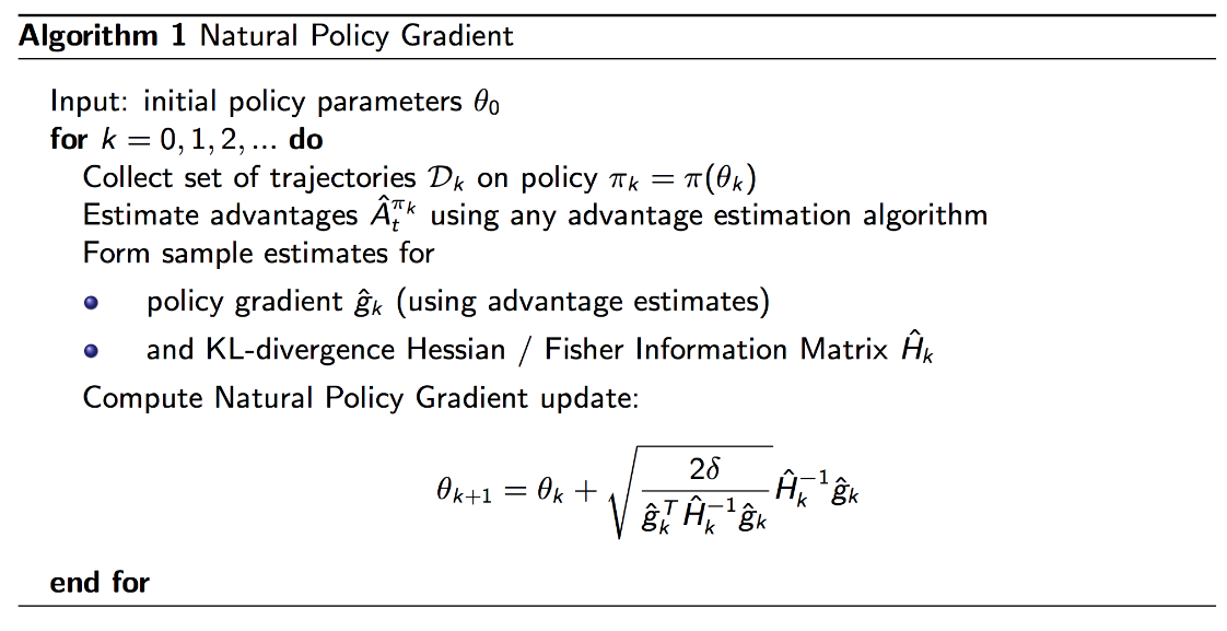
Pseudocode

Implementation

import tensorflow.compat.v1 as tf
tf.disable_v2_behavior() # to make it possible to run 1.X code in tf2
import numpy as np
import gym
import random

def policy_gradient():
    with tf.variable_scope("policy"):
        params = tf.get_variable("policy_parameters", [4, 2])
        state = tf.placeholder("float", [None, 4], name="state")
        # NOTE: have to specify shape of actions so we can call
        # get_shape when calculating g_log_prob below
        actions = tf.placeholder("float", [200, 2], name="actions")
        advantages = tf.placeholder("float", [None,], name="advantages")
        linear = tf.matmul(state, params) #shape: [None, 2]
        probabilities = tf.nn.softmax(linear) #shape: [None, 2]
        my_variables = tf.trainable_variables()

        # calculate the probability of the chosen action given the state
        # shape: [200, 2] ---> [1, 2] the probs of two actions
        action_log_prob = tf.log(tf.reduce_sum(
            tf.multiply(probabilities, actions), reduction_indices=[1]))

        # calculate the gradient of the log probability at each point in time
        # NOTE: doing this because tf.gradients only returns a summed version
        action_log_prob_flat = tf.reshape(action_log_prob, (-1,)) #shape:(2,)

        g_log_prob = tf.stack(
            [tf.gradients(action_log_prob_flat[i], my_variables)[0]
             for i in range(action_log_prob_flat.get_shape()[0])])
        g_log_prob = tf.reshape(g_log_prob, (200, 8, 1))

        # calculate the policy gradient by multiplying by the advantage function
        # shape:(200, 8, 1)
        g = tf.multiply(g_log_prob, tf.reshape(advantages, (200, 1, 1)))
        # sum over time
        g = 1.00 / 200.00 * tf.reduce_sum(g, reduction_indices=[0]) #shape:(8, 1)

        F2 = tf.map_fn(lambda x: tf.matmul(x, tf.transpose(x)), g_log_prob)
        F = 1.0 / 200.00 * tf.reduce_sum(F2, reduction_indices=[0]) #T=200

        # calculate inverse of positive definite clipped F
        # NOTE: have noticed small eigenvalues (1e-10) that are negative,
        # using SVD to clip those out, assuming they're rounding errors
        S, U, V = tf.svd(F)
        atol = tf.reduce_max(S) * 1e-6
        S_inv = tf.divide(1.0, S)
        S_inv = tf.where(S < atol, tf.zeros_like(S), S_inv)
        S_inv = tf.diag(S_inv)
        F_inv = tf.matmul(S_inv, tf.transpose(U))
        F_inv = tf.matmul(V, F_inv)

        # calculate natural policy gradient ascent update
        F_inv_g = tf.matmul(F_inv, g)
        # calculate a learning rate normalized such that a constant change
        # in the output control policy is achieved each update, preventing
        # any parameter changes that hugely change the output
        learning_rate = tf.sqrt(tf.divide(0.001, tf.matmul(tf.transpose(g), F_inv_g)))

        update = tf.multiply(learning_rate, F_inv_g)
        update = tf.reshape(update, (4, 2))

        # update trainable parameters
        # NOTE: whenever my_variables is fetched they're also updated
        my_variables[0] = tf.assign_add(my_variables[0], update)

        return probabilities, state, actions, advantages, my_variables

def value_gradient():
    with tf.variable_scope("value"):
        state = tf.placeholder("float", [None, 4])
        new_vals = tf.placeholder("float", [None, 1])
        w1 = tf.get_variable("w1", [4, 10])
        b1 = tf.get_variable("b1", [10])
        h1 = tf.nn.relu(tf.matmul(state, w1) + b1)
        w2 = tf.get_variable("w2", [10, 1])
        b2 = tf.get_variable("b2", [1])
        calculated = tf.matmul(h1, w2) + b2

        # minimize the difference between predicted and actual
        diffs = calculated - new_vals
        loss = tf.nn.l2_loss(diffs)
        optimizer = tf.train.AdamOptimizer(0.1).minimize(loss)

        return calculated, state, new_vals, optimizer, loss

def run_episode(env, policy_grad, value_grad, sess):
    # unpack the policy network (generates control policy)
    (pl_calculated, pl_state, pl_actions, pl_advantages, pl_optimizer) = policy_grad
    # unpack the value network (estimates expected reward)
    (vl_calculated, vl_state, vl_new_vals, vl_optimizer, vl_loss) = value_grad
    # set up the environment
    observation = env.reset() #shape:(4,)

    episode_reward = 0
    total_rewards = []
    states = []
    actions =[]
    advantages = []
    transitions = []
    update_vals = []

    n_episodes = 0
    n_timesteps = 200
    for t in range(n_timesteps):
        # calculate policy
        obs_vector = np.expand_dims(observation, axis=0) #shape:(1, 4)
        probs = sess.run(pl_calculated, feed_dict={pl_state: obs_vector})
        # stochastically generate action using the policy output
        action = 0 if random.uniform(0, 1) < probs[0][0] else 1
        # record the transition
        states.append(observation)
        action_blank = np.zeros(2)
        action_blank[action] = 1
        actions.append(action_blank)
        # take the action in the environment
        old_observation = observation
        observation, reward, done, info = env.step(action)
        transitions.append((old_observation, action, reward))
        episode_reward += reward

        # if the pole falls or time is up
        if done or t == n_timesteps - 1:
            for ii, trans in enumerate(transitions):
                obs, action, reward = trans
                # calculate discounted monte-carlo return
                future_reward = 0
                future_transitions = len(transitions) - ii
                decrease = 1
                for jj in range(future_transitions):
                    future_reward += transitions[jj + ii][2] * decrease
                    decrease = decrease * 0.97
                obs_vector = np.expand_dims(obs, axis=0)
                # compare the calculated expected reward to the average
                # expected reward, as estimated by the value network
                current_val = sess.run(vl_calculated, feed_dict={
                    vl_state: obs_vector})[0][0]
                # advantage: how much better was this action than normal
                advantages.append(future_reward - current_val)
                # update the value function towards new return
                update_vals.append(future_reward)

            n_episodes += 1
            # reset variables for next episode in batch
            total_rewards.append(episode_reward)
            episode_reward = 0.0
            transitions = []

            if done:
                # if the pole fell, reset environment
                observation = env.reset()
            else:
                # if out of time, close environment
                env.close()

    print("total_rewards: ", total_rewards)

    # update value function
    update_vals_vector = np.expand_dims(update_vals, axis=1)
    sess.run(vl_optimizer, feed_dict={vl_state: states, vl_new_vals: update_vals_vector})
    # update control policy
    sess.run(pl_optimizer, feed_dict={
        pl_state: states, pl_advantages: advantages, pl_actions: actions})
    return total_rewards, n_episodes

# generate the networks
policy_grad = policy_gradient()
value_grad = value_gradient()

# run the training from scratch 10 times, record results
for ii in range(10): #ran 10 sessions of 300 batches
    env = gym.make("CartPole-v0")
    # env = gym.wrappers.Monitor(env=env, directory="./", force=True, video_callable=False)
    sess = tf.InteractiveSession()
    sess.run(tf.global_variables_initializer())

    max_rewards = []
    total_episodes = []
    # each batch is 200 time steps worth of episodes
    n_training_batches = 300
    times = []
    for i in range(n_training_batches):
        if i % 100 == 0:
            print(i)
        reward, n_episodes = run_episode(env, policy_grad, value_grad, sess)
        max_rewards.append(np.max(reward))
        total_episodes.append(n_episodes)
    sess.close()

100

101

102

103

104

105

106

107

108

109

110

111

112

113

114

115

116

117

118

119

120

121

122

123

124

125

126

127

128

129

130

131

132

133

134

135

136

137

138

139

140

141

142

143

144

145

146

147

148

149

150

151

152

153

154

155

156

157

158

159

160

161

162

163

164

165

166

167

168

169

170

171

172

173

174

175

176

177

178

179

180

181

182

183

184

185

186

187

188

import tensorflow.compat.v1 as tf

tf.disable_v2_behavior() # to make it possible to run 1.X code in tf2

import numpy as np

import gym

import random

def policy_gradient():

with tf.variable_scope("policy"):

params = tf.get_variable("policy_parameters", [4, 2])

state = tf.placeholder("float", [None, 4], name="state")

# NOTE: have to specify shape of actions so we can call

# get_shape when calculating g_log_prob below

actions = tf.placeholder("float", [200, 2], name="actions")

advantages = tf.placeholder("float", [None,], name="advantages")

linear = tf.matmul(state, params) #shape: [None, 2]

probabilities = tf.nn.softmax(linear) #shape: [None, 2]

my_variables = tf.trainable_variables()

# calculate the probability of the chosen action given the state

# shape: [200, 2] ---> [1, 2] the probs of two actions

action_log_prob = tf.log(tf.reduce_sum(

tf.multiply(probabilities, actions), reduction_indices=[1]))

# calculate the gradient of the log probability at each point in time

# NOTE: doing this because tf.gradients only returns a summed version

action_log_prob_flat = tf.reshape(action_log_prob, (-1,)) #shape:(2,)

g_log_prob = tf.stack(

[tf.gradients(action_log_prob_flat[i], my_variables)[0]

for i in range(action_log_prob_flat.get_shape()[0])])

g_log_prob = tf.reshape(g_log_prob, (200, 8, 1))

# calculate the policy gradient by multiplying by the advantage function

# shape:(200, 8, 1)

g = tf.multiply(g_log_prob, tf.reshape(advantages, (200, 1, 1)))

# sum over time

g = 1.00 / 200.00 * tf.reduce_sum(g, reduction_indices=[0]) #shape:(8, 1)

F2 = tf.map_fn(lambda x: tf.matmul(x, tf.transpose(x)), g_log_prob)

F = 1.0 / 200.00 * tf.reduce_sum(F2, reduction_indices=[0]) #T=200

# calculate inverse of positive definite clipped F

# NOTE: have noticed small eigenvalues (1e-10) that are negative,

# using SVD to clip those out, assuming they're rounding errors

S, U, V = tf.svd(F)

atol = tf.reduce_max(S) * 1e-6

S_inv = tf.divide(1.0, S)

S_inv = tf.where(S < atol, tf.zeros_like(S), S_inv)

S_inv = tf.diag(S_inv)

F_inv = tf.matmul(S_inv, tf.transpose(U))

F_inv = tf.matmul(V, F_inv)

# calculate natural policy gradient ascent update

F_inv_g = tf.matmul(F_inv, g)

# calculate a learning rate normalized such that a constant change

# in the output control policy is achieved each update, preventing

# any parameter changes that hugely change the output

learning_rate = tf.sqrt(tf.divide(0.001, tf.matmul(tf.transpose(g), F_inv_g)))

update = tf.multiply(learning_rate, F_inv_g)

update = tf.reshape(update, (4, 2))

# update trainable parameters

# NOTE: whenever my_variables is fetched they're also updated

my_variables[0] = tf.assign_add(my_variables[0], update)

return probabilities, state, actions, advantages, my_variables

def value_gradient():

with tf.variable_scope("value"):

state = tf.placeholder("float", [None, 4])

new_vals = tf.placeholder("float", [None, 1])

w1 = tf.get_variable("w1", [4, 10])

b1 = tf.get_variable("b1", [10])

h1 = tf.nn.relu(tf.matmul(state, w1) + b1)

w2 = tf.get_variable("w2", [10, 1])

b2 = tf.get_variable("b2", [1])

calculated = tf.matmul(h1, w2) + b2

# minimize the difference between predicted and actual

diffs = calculated - new_vals

loss = tf.nn.l2_loss(diffs)

optimizer = tf.train.AdamOptimizer(0.1).minimize(loss)

return calculated, state, new_vals, optimizer, loss

def run_episode(env, policy_grad, value_grad, sess):

# unpack the policy network (generates control policy)

(pl_calculated, pl_state, pl_actions, pl_advantages, pl_optimizer) = policy_grad

# unpack the value network (estimates expected reward)

(vl_calculated, vl_state, vl_new_vals, vl_optimizer, vl_loss) = value_grad

# set up the environment

observation = env.reset() #shape:(4,)

episode_reward = 0

total_rewards = []

states = []

actions =[]

advantages = []

transitions = []

update_vals = []

n_episodes = 0

n_timesteps = 200

for t in range(n_timesteps):

# calculate policy

obs_vector = np.expand_dims(observation, axis=0) #shape:(1, 4)

probs = sess.run(pl_calculated, feed_dict={pl_state: obs_vector})

# stochastically generate action using the policy output

action = 0 if random.uniform(0, 1) < probs[0][0] else 1

# record the transition

states.append(observation)

action_blank = np.zeros(2)

action_blank[action] = 1

actions.append(action_blank)

# take the action in the environment

old_observation = observation

observation, reward, done, info = env.step(action)

transitions.append((old_observation, action, reward))

episode_reward += reward

# if the pole falls or time is up

if done or t == n_timesteps - 1:

for ii, trans in enumerate(transitions):

obs, action, reward = trans

# calculate discounted monte-carlo return

future_reward = 0

future_transitions = len(transitions) - ii

decrease = 1

for jj in range(future_transitions):

future_reward += transitions[jj + ii][2] * decrease

decrease = decrease * 0.97

obs_vector = np.expand_dims(obs, axis=0)

# compare the calculated expected reward to the average

# expected reward, as estimated by the value network

current_val = sess.run(vl_calculated, feed_dict={

vl_state: obs_vector})[0][0]

# advantage: how much better was this action than normal

advantages.append(future_reward - current_val)

# update the value function towards new return

update_vals.append(future_reward)

n_episodes += 1

# reset variables for next episode in batch

total_rewards.append(episode_reward)

episode_reward = 0.0

transitions = []

if done:

# if the pole fell, reset environment

observation = env.reset()

else:

# if out of time, close environment

env.close()

print("total_rewards: ", total_rewards)

# update value function

update_vals_vector = np.expand_dims(update_vals, axis=1)

sess.run(vl_optimizer, feed_dict={vl_state: states, vl_new_vals: update_vals_vector})

# update control policy

sess.run(pl_optimizer, feed_dict={

pl_state: states, pl_advantages: advantages, pl_actions: actions})

return total_rewards, n_episodes

# generate the networks

policy_grad = policy_gradient()

value_grad = value_gradient()

# run the training from scratch 10 times, record results

for ii in range(10): #ran 10 sessions of 300 batches

env = gym.make("CartPole-v0")

# env = gym.wrappers.Monitor(env=env, directory="./", force=True, video_callable=False)

sess = tf.InteractiveSession()

sess.run(tf.global_variables_initializer())

max_rewards = []

total_episodes = []

# each batch is 200 time steps worth of episodes

n_training_batches = 300

times = []

for i in range(n_training_batches):

if i % 100 == 0:

print(i)

reward, n_episodes = run_episode(env, policy_grad, value_grad, sess)

max_rewards.append(np.max(reward))

total_episodes.append(n_episodes)

sess.close()

Results

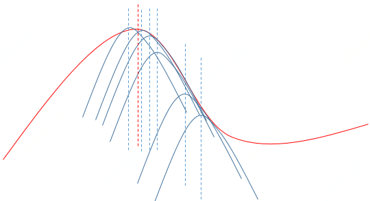
5. Summary

I will end the post with a summary graph as bellow to connection between different parts of the Natural Gradient as bellow

1. Minorize-Maximization, MM

2. Fisher Information Matrix

3. Fisher Information Matrix and KL-divergence

4. Natural Policy Gradient

5. Summary

Leave a Reply Cancel reply