Policy gradient methods have advantages over better convergence properties, being effective in high-dimensional or continuous action spaces and being able to learn stochastic policies.
1. Policy-based Methods
In value-based approaches, in order to learn a policy, we must find the optimal state value function or state-action value function with parameters  ,
,
![\[\begin{array}{l}{V_\theta }\left( s \right) \approx {V^{\rm{\pi }}}\left( s \right)\\{Q_\theta }\left( {s,a} \right) \approx {Q^{\rm{\pi }}}\left( {s,a} \right)\end{array}\]](http://www.liaoyong.net/wp-content/ql-cache/quicklatex.com-be8e7bb3531d140edfa84e7e21fbc531_l3.png "Rendered by QuickLaTeX.com")
 or
or  to extract a policy, e.g. with
  -greedy.
Why not learn the policy directly? The policy-based methods parameterize the policy directly:
![\[{{\rm{\pi }}_\theta }\left( {a\left| s \right.} \right) = \mathbb{P}\left[ {a\left| s \right.;\theta } \right]\]](http://www.liaoyong.net/wp-content/ql-cache/quicklatex.com-9fcb93c66b5011682d0031f0ac351f5d_l3.png "Rendered by QuickLaTeX.com")
We focus on the basic and widely used gradient-based algorithm REINFORCE and VPG here to present main ideas, process and how they are used to solve practical reinforcement learning problems.
2. Policy Gradient
The object function of the reinforcement learning algorithm is:
![\[J\left( \theta \right) = {\mathbb{E}_{\tau \sim {{\rm{\pi }}_\theta }\left( \tau \right)}}\left[ {\sum\limits_t {{\gamma ^t}r\left( {{s_t},{a_t}} \right)} } \right] = \int {{{\rm{\pi }}_\theta }\left( \tau \right)r\left( \tau \right)d\tau } \approx \frac{1}{N}\sum\limits_{i = 1}^N {\sum\limits_{t = 1}^T {{\gamma ^t}r\left( {{s_t},{a_t}} \right)} } \]](http://www.liaoyong.net/wp-content/ql-cache/quicklatex.com-28c6a1ed906d7ff2cd8eebbec6ef43ae_l3.png "Rendered by QuickLaTeX.com")
 can be approximated by sampling different trajectories and calculate the corresponding average. The goal of the agent or learned policy to maximize :
 ![\[{\theta ^*} = \mathop {\arg \max }\limits_\theta J\left( \theta \right)\]](http://www.liaoyong.net/wp-content/ql-cache/quicklatex.com-c65e0fc1d7ae4c8c30bec7c032fd9f48_l3.png "Rendered by QuickLaTeX.com")
![\[\begin{array}{l}{{\rm{\pi }}_\theta }\left( \tau \right) = {{\rm{\pi }}_\theta }\left( {{s_1},{a_1}, \cdots ,{s_T},{a_T}} \right) = p\left( {{s_1}} \right)\prod\limits_{t = 1}^T {{{\rm{\pi }}_\theta }\left( {{a_t}\left| {{s_t}} \right.} \right)} p\left( {{s_{t + 1}}\left| {{s_t},{a_t}} \right.} \right)\\\log {{\rm{\pi }}_\theta }\left( \tau \right) = \log p\left( {{s_1}} \right) + \sum\limits_{t = 1}^T {\left[ {\log {{\rm{\pi }}_\theta }\left( {{a_t}\left| {{s_t}} \right.} \right) + \log p\left( {{s_{t + 1}}\left| {{s_t},{a_t}} \right.} \right)} \right]} \end{array}\]](http://www.liaoyong.net/wp-content/ql-cache/quicklatex.com-2deb0486f698996c5c1b73ed224a74d2_l3.png "Rendered by QuickLaTeX.com")
![\[\begin{array}{l}{\nabla _\theta }J\left( \theta \right) = \int {{\nabla _\theta }{{\rm{\pi }}_\theta }\left( \tau \right)r\left( \tau \right)d\tau } \\{\kern 1pt} {\kern 1pt} {\kern 1pt} {\kern 1pt} {\kern 1pt} {\kern 1pt} {\kern 1pt} {\kern 1pt} {\kern 1pt} {\kern 1pt} {\kern 1pt} {\kern 1pt} {\kern 1pt} {\kern 1pt} {\kern 1pt} {\kern 1pt} {\kern 1pt} {\kern 1pt} {\kern 1pt} {\kern 1pt} {\kern 1pt} {\kern 1pt} {\kern 1pt} {\kern 1pt} {\kern 1pt} {\kern 1pt} {\kern 1pt} {\kern 1pt} {\kern 1pt} {\kern 1pt} {\kern 1pt} {\kern 1pt} {\kern 1pt} {\kern 1pt} {\kern 1pt} {\kern 1pt} {\kern 1pt} {\kern 1pt} = \int {{{\rm{\pi }}_\theta }\left( \tau \right)\frac{{{\nabla _\theta }{{\rm{\pi }}_\theta }\left( \tau \right)}}{{{{\rm{\pi }}_\theta }\left( \tau \right)}}r\left( \tau \right)d\tau } \\{\kern 1pt} {\kern 1pt} {\kern 1pt} {\kern 1pt} {\kern 1pt} {\kern 1pt} {\kern 1pt} {\kern 1pt} {\kern 1pt} {\kern 1pt} {\kern 1pt} {\kern 1pt} {\kern 1pt} {\kern 1pt} {\kern 1pt} {\kern 1pt} {\kern 1pt} {\kern 1pt} {\kern 1pt} {\kern 1pt} {\kern 1pt} {\kern 1pt} {\kern 1pt} {\kern 1pt} {\kern 1pt} {\kern 1pt} {\kern 1pt} {\kern 1pt} {\kern 1pt} {\kern 1pt} {\kern 1pt} {\kern 1pt} {\kern 1pt} {\kern 1pt} {\kern 1pt} {\kern 1pt} {\kern 1pt} {\kern 1pt} {\kern 1pt} = \int {{{\rm{\pi }}_\theta }\left( \tau \right){\nabla _\theta }\log {{\rm{\pi }}_\theta }\left( \tau \right)r\left( \tau \right)d\tau } \\{\kern 1pt} {\kern 1pt} {\kern 1pt} {\kern 1pt} {\kern 1pt} {\kern 1pt} {\kern 1pt} {\kern 1pt} {\kern 1pt} {\kern 1pt} {\kern 1pt} {\kern 1pt} {\kern 1pt} {\kern 1pt} {\kern 1pt} {\kern 1pt} {\kern 1pt} {\kern 1pt} {\kern 1pt} {\kern 1pt} {\kern 1pt} {\kern 1pt} {\kern 1pt} {\kern 1pt} {\kern 1pt} {\kern 1pt} {\kern 1pt} {\kern 1pt} {\kern 1pt} {\kern 1pt} {\kern 1pt} {\kern 1pt} {\kern 1pt} {\kern 1pt} {\kern 1pt} {\kern 1pt} {\kern 1pt} {\kern 1pt} = {\mathbb{E}_{\tau \sim {{\rm{\pi }}_\theta }\left( \tau \right)}}\left[ {{\nabla _\theta }\log {{\rm{\pi }}_\theta }\left( \tau \right)r\left( \tau \right)} \right]\end{array}\]](http://www.liaoyong.net/wp-content/ql-cache/quicklatex.com-2c90ce5c0e49c6d81a12f70c555d1c01_l3.png "Rendered by QuickLaTeX.com")
with respect to can be written as: ![\[\begin{array}{l}{\nabla _\theta }J\left( \theta \right) = {\mathbb{E}_{\tau \sim {{\rm{\pi }}_\theta }\left( \tau \right)}}\left[ {{\nabla _\theta }\log {{\rm{\pi }}_\theta }\left( \tau \right)r\left( \tau \right)} \right]\\{\kern 1pt} {\kern 1pt} {\kern 1pt} {\kern 1pt} {\kern 1pt} {\kern 1pt} {\kern 1pt} {\kern 1pt} {\kern 1pt} {\kern 1pt} {\kern 1pt} {\kern 1pt} {\kern 1pt} {\kern 1pt} {\kern 1pt} {\kern 1pt} {\kern 1pt} {\kern 1pt} {\kern 1pt} {\kern 1pt} {\kern 1pt} {\kern 1pt} {\kern 1pt} {\kern 1pt} {\kern 1pt} {\kern 1pt} {\kern 1pt} {\kern 1pt} {\kern 1pt} {\kern 1pt} {\kern 1pt} {\kern 1pt} {\kern 1pt} {\kern 1pt} {\kern 1pt} {\kern 1pt} {\kern 1pt} {\kern 1pt} {\kern 1pt} {\kern 1pt} = {\mathbb{E}_{\tau \sim {{\rm{\pi }}_\theta }\left( \tau \right)}}\left[ {{\nabla _\theta }\left[ {\log p\left( {{s_1}} \right) + \sum\limits_{t = 1}^T {\left( {\log {{\rm{\pi }}_\theta }\left( {{a_t}\left| {{s_t}} \right.} \right) + \log p\left( {{s_{t + 1}}\left| {{s_t},{a_t}} \right.} \right)} \right)} } \right]r\left( \tau \right)} \right]\\{\kern 1pt} {\kern 1pt} {\kern 1pt} {\kern 1pt} {\kern 1pt} {\kern 1pt} {\kern 1pt} {\kern 1pt} {\kern 1pt} {\kern 1pt} {\kern 1pt} {\kern 1pt} {\kern 1pt} {\kern 1pt} {\kern 1pt} {\kern 1pt} {\kern 1pt} {\kern 1pt} {\kern 1pt} {\kern 1pt} {\kern 1pt} {\kern 1pt} {\kern 1pt} {\kern 1pt} {\kern 1pt} {\kern 1pt} {\kern 1pt} {\kern 1pt} {\kern 1pt} {\kern 1pt} {\kern 1pt} {\kern 1pt} {\kern 1pt} {\kern 1pt} {\kern 1pt} {\kern 1pt} {\kern 1pt} {\kern 1pt} {\kern 1pt} = {\mathbb{E}_{\tau \sim {{\rm{\pi }}_\theta }\left( \tau \right)}}\left[ {{\nabla _\theta }\left[ {\sum\limits_{t = 1}^T {\log {{\rm{\pi }}_\theta }\left( {{a_t}\left| {{s_t}} \right.} \right)} } \right]r\left( \tau \right)} \right]\\{\kern 1pt} {\kern 1pt} {\kern 1pt} {\kern 1pt} {\kern 1pt} {\kern 1pt} {\kern 1pt} {\kern 1pt} {\kern 1pt} {\kern 1pt} {\kern 1pt} {\kern 1pt} {\kern 1pt} {\kern 1pt} {\kern 1pt} {\kern 1pt} {\kern 1pt} {\kern 1pt} {\kern 1pt} {\kern 1pt} {\kern 1pt} {\kern 1pt} {\kern 1pt} {\kern 1pt} {\kern 1pt} {\kern 1pt} {\kern 1pt} {\kern 1pt} {\kern 1pt} {\kern 1pt} {\kern 1pt} {\kern 1pt} {\kern 1pt} {\kern 1pt} {\kern 1pt} {\kern 1pt} {\kern 1pt} {\kern 1pt} {\kern 1pt} = {\mathbb{E}_{\tau \sim {{\rm{\pi }}_\theta }\left( \tau \right)}}\left[ {\sum\limits_{t = 1}^T {\left( {{\nabla _\theta }\left( {\log {{\rm{\pi }}_\theta }\left( {{a_t}\left| {{s_t}} \right.} \right)} \right)\left( {\sum\limits_{t = 1}^T {{\gamma ^t}r\left( {{s_t},{a_t}} \right)} } \right)} \right)} } \right]\\{\kern 1pt} {\kern 1pt} {\kern 1pt} {\kern 1pt} {\kern 1pt} {\kern 1pt} {\kern 1pt} {\kern 1pt} {\kern 1pt} {\kern 1pt} {\kern 1pt} {\kern 1pt} {\kern 1pt} {\kern 1pt} {\kern 1pt} {\kern 1pt} {\kern 1pt} {\kern 1pt} {\kern 1pt} {\kern 1pt} {\kern 1pt} {\kern 1pt} {\kern 1pt} {\kern 1pt} {\kern 1pt} {\kern 1pt} {\kern 1pt} {\kern 1pt} {\kern 1pt} {\kern 1pt} {\kern 1pt} {\kern 1pt} {\kern 1pt} {\kern 1pt} {\kern 1pt} {\kern 1pt} {\kern 1pt} {\kern 1pt} \approx \frac{1}{N}\sum\limits_{i = 1}^N {\left[ {\underline {\sum\limits_{t = 1}^T {\left( {\underline {{\nabla _\theta }\left( {\log {{\rm{\pi }}_\theta }\left( {{a_{i,t}}\left| {{s_{i,t}}} \right.} \right)} \right)\left( {\sum\limits_{t = 1}^T {\underline {{\gamma ^t}r\left( {{s_{i,t}},{a_{i,t}}} \right)} } } \right)} } \right)} } } \right]} \end{array}\]](http://www.liaoyong.net/wp-content/ql-cache/quicklatex.com-8b6ea17eb866c7e0d2fe4a2fab71313e_l3.png "Rendered by QuickLaTeX.com")
 takes no effect to actions before time , above formula is equivalent to:
 ![\[{\nabla _\theta }J\left( \theta \right) \approx \frac{1}{N}\sum\limits_{i = 1}^N {\sum\limits_{t = 1}^T {\left[ {{\nabla _\theta }\log {{\rm{\pi }}_\theta }\left( {{a_{i,t}}\left| {{s_{i,t}}} \right.} \right)\left( {\underline {\sum\limits_{t' = t}^T {{\gamma ^t}r\left( {{s_{i,t'}},{a_{i,t'}}} \right)} } } \right)} \right]} } = \frac{1}{N}\sum\limits_{i = 1}^N {\sum\limits_{t = 1}^T {\left[ {{\nabla _\theta }\log {{\rm{\pi }}_\theta }\left( {{a_{i,t}}\left| {{s_{i,t}}} \right.} \right){{\hat Q}_{i,t}}} \right]} } \]](http://www.liaoyong.net/wp-content/ql-cache/quicklatex.com-b007e98b58d60c7b4596d23de665da4d_l3.png "Rendered by QuickLaTeX.com")
 is just
  function according to its definition. Meanwhile, by changing
  to
to  , the number of
  term is reduced, thus leading to the variance reduction.
Furthermore, the base-line
 is introduced to reduce high variance.
 ![\[{\nabla _\theta }J\left( \theta \right) \approx \frac{1}{N}\sum\limits_{i = 1}^N {\sum\limits_{t = 1}^T {\left[ {{\nabla _\theta }\log {{\rm{\pi }}_\theta }\left( {{a_{i,t}}\left| {{s_{i,t}}} \right.} \right)\left( {\sum\limits_{t' = t}^T {{\gamma ^t}r\left( {{s_{i,t'}},{a_{i,t'}}} \right)} - b} \right)} \right]} } \]](http://www.liaoyong.net/wp-content/ql-cache/quicklatex.com-d0a2ed72d2b47a4f7aed3eb09688884d_l3.png "Rendered by QuickLaTeX.com")
is the value function  , thus we get
 ![\[A = \sum\limits_{t' = t}^T {{\gamma ^t}r\left( {{s_{i,t'}},{a_{i,t'}}} \right)} - b = Q - V\]](http://www.liaoyong.net/wp-content/ql-cache/quicklatex.com-8076c7322f3e8c8bbc7249556f7a3e08_l3.png "Rendered by QuickLaTeX.com")
 is the advantage function, meaning how much better it is for the agent to take the action
  in a state
  than the average. An analytical solution for optimal baseline is
 ![\[b = \frac{{\mathbb{E}\left[ {{{\left( {{\nabla _\theta }\log {{\rm{\pi }}_\theta }\left( \tau \right)} \right)}^2}r\left( \tau \right)} \right]}}{{\mathbb{E}\left[ {{{\left( {{\nabla _\theta }\log {{\rm{\pi }}_\theta }\left( \tau \right)} \right)}^2}} \right]}}\]](http://www.liaoyong.net/wp-content/ql-cache/quicklatex.com-6d0b7e04cc84e146cf5a0fbbab9ee208_l3.png "Rendered by QuickLaTeX.com")
The key idea underlying policy gradients is to push up the probabilities of actions that lead to higher return, and push down the probabilities of actions that lead to lower return, until you arrive at the optimal policy.
3. REINFORCE
The REINFORCE algorithm is also called Monte-Carlo Policy Gradient Algorithm. It samples multiple trajectories following the policy  and updates using the estimated gradient by these samples. The update rule is as follow:
![\[\begin{array}{l}{\nabla _\theta }J\left( \theta \right) \approx \frac{1}{N}\sum\limits_{i = 1}^N {\left[ {\sum\limits_{t = 1}^T {\left( {{\nabla _\theta }\left( {\log {{\rm{\pi }}_\theta }\left( {{a_{i,t}}\left| {{s_{i,t}}} \right.} \right)} \right)\left( {\sum\limits_{t = 1}^T {{\gamma ^t}r\left( {{s_{i,t}},{a_{i,t}}} \right)} } \right)} \right)} } \right]} \\{\kern 1pt} {\kern 1pt} {\kern 1pt} {\kern 1pt} {\kern 1pt} {\kern 1pt} {\kern 1pt} {\kern 1pt} {\kern 1pt} {\kern 1pt} {\kern 1pt} {\kern 1pt} {\kern 1pt} {\kern 1pt} {\kern 1pt} {\kern 1pt} {\kern 1pt} {\kern 1pt} {\kern 1pt} {\kern 1pt} {\kern 1pt} {\kern 1pt} {\kern 1pt} {\kern 1pt} {\kern 1pt} {\kern 1pt} {\kern 1pt} {\kern 1pt} {\kern 1pt} {\kern 1pt} {\kern 1pt} {\kern 1pt} {\kern 1pt} {\kern 1pt} {\kern 1pt} {\kern 1pt} {\kern 1pt} {\kern 1pt} {\kern 1pt} \approx \frac{1}{N}\sum\limits_{i = 1}^N {\left[ {\sum\limits_{t = 1}^T {\left( {{\nabla _\theta }\log {{\rm{\pi }}_\theta }\left( {{a_{i,t}}\left| {{s_{i,t}}} \right.} \right){G_{i,t}}} \right)} } \right]} {\kern 1pt} {\kern 1pt} \end{array}\]](http://www.liaoyong.net/wp-content/ql-cache/quicklatex.com-9082e7aa16b5eda5df61cdb061665d93_l3.png "Rendered by QuickLaTeX.com")
 Code implementation:
|
1 2 3 4 5 6 7 8 9 10 11 12 13 14 15 16 17 18 19 20 21 22 23 24 25 26 27 28 29 30 31 32 33 34 35 36 37 38 39 40 41 42 43 44 45 46 47 48 49 50 51 52 53 54 55 56 57 58 59 60 61 62 63 64 65 66 67 68 69 70 71 72 73 74 75 76 77 78 79 80 81 82 83 84 85 86 87 88 89 90 91 92 93 94 95 96 97 98 99 100 101 102 103 104 105 106 107 108 109 110 111 112 113 114 115 116 117 118 119 120 121 122 123 124 125 126 127 128 129 130 131 132 133 134 135 136 137 138 139 140 141 142 143 144 145 |
import sys import gym import numpy as np import matplotlib.pyplot as plt from keras.layers import Dense from keras.models import Sequential from keras.optimizers import Adam EPISODES = 1000 # This is Policy Gradient agent for the Cartpole # In this example, we use REINFORCE algorithm which uses monte-carlo update rule class REINFORCEAgent: def __init__(self, state_size, action_size): # if you want to see Cartpole learning, then change to True self.render = False self.load_model = False # get size of state and action self.state_size = state_size self.action_size = action_size # These are hyper parameters for the Policy Gradient self.discount_factor = 0.99 self.learning_rate = 0.001 self.hidden1, self.hidden2 = 24, 24 # create model for policy network self.model = self.build_model() # lists for the states, actions and rewards self.states, self.actions, self.rewards = [], [], [] if self.load_model: self.model.load_weights("./save_model/cartpole_reinforce.h5") # approximate policy using Neural Network # state is input and probability of each action is output of network def build_model(self): model = Sequential() model.add( Dense(self.hidden1, input_dim=self.state_size, activation='relu', kernel_initializer='glorot_uniform')) model.add(Dense(self.hidden2, activation='relu', kernel_initializer='glorot_uniform')) model.add(Dense(self.action_size, activation='softmax', kernel_initializer='glorot_uniform')) model.summary() # Using categorical crossentropy as a loss is a trick to easily # implement the policy gradient. Categorical cross entropy is defined # H(p, q) = sum(p_i * log(q_i)). For the action taken, a, you set # p_a = advantage. q_a is the output of the policy network, which is # the probability of taking the action a, i.e. policy(s, a). # All other p_i are zero, thus we have H(p, q) = A * log(policy(s, a)) model.compile(loss="categorical_crossentropy", optimizer=Adam(lr=self.learning_rate)) return model # using the output of policy network, pick action stochastically def get_action(self, state): policy = self.model.predict(state, batch_size=1).flatten() return np.random.choice(self.action_size, 1, p=policy)[0] # In Policy Gradient, Q function is not available. # Instead agent uses sample returns for evaluating policy def discount_rewards(self, rewards): discounted_rewards = np.zeros_like(rewards) running_add = 0 for t in reversed(range(0, len(rewards))): running_add = running_add * self.discount_factor + rewards[t] discounted_rewards[t] = running_add return discounted_rewards # save <s, a ,r> of each step def append_sample(self, state, action, reward): self.states.append(state) self.rewards.append(reward) self.actions.append(action) # update policy network every episode def train_model(self): episode_length = len(self.states) discounted_rewards = self.discount_rewards(self.rewards) discounted_rewards -= np.mean(discounted_rewards) discounted_rewards /= np.std(discounted_rewards) update_inputs = np.zeros((episode_length, self.state_size)) advantages = np.zeros((episode_length, self.action_size)) for i in range(episode_length): update_inputs[i] = self.states[i] advantages[i][self.actions[i]] = discounted_rewards[i] self.model.fit(update_inputs, advantages, epochs=1, verbose=0) self.states, self.actions, self.rewards = [], [], [] if __name__ == "__main__": # In case of CartPole-v1, you can play until 500 time step env = gym.make('CartPole-v1') # get size of state and action from environment state_size = env.observation_space.shape[0] action_size = env.action_space.n # make REINFORCE agent agent = REINFORCEAgent(state_size, action_size) scores, episodes = [], [] for e in range(EPISODES): done = False score = 0 state = env.reset() state = np.reshape(state, [1, state_size]) while not done: if agent.render: env.render() # get action for the current state and go one step in environment action = agent.get_action(state) next_state, reward, done, info = env.step(action) next_state = np.reshape(next_state, [1, state_size]) reward = reward if not done or score == 499 else -100 # save the sample <s, a, r> to the memory agent.append_sample(state, action, reward) score += reward state = next_state if done: # every episode, agent learns from sample returns agent.train_model() # every episode, plot the play time score = score if score == 500 else score + 100 scores.append(score) episodes.append(e) plt.plot(episodes, scores, 'b') plt.savefig("./save_graph/cartpole_reinforce.png") print("episode:", e, " score:", score) # if the mean of scores of last 10 episode is bigger than 490 # stop training if np.mean(scores[-min(10, len(scores)):]) > 490: sys.exit() # save the model if e % 50 == 0: agent.model.save_weights("./save_model/cartpole_reinforce.h5") |
4. Vanilla Policy Gradient
REINFORCE algorithm using  for gradient estimation is often of high variance across multiple episodes. According to the above session, subtracting a baseline
  from may help to reduce the variance as long as the baseline does not vary with the action .
![\[{\kern 1pt} {\kern 1pt} {\nabla _\theta }J\left( \theta \right) \approx \frac{1}{N}\sum\limits_{i = 1}^N {\left[ {\sum\limits_{t = 1}^T {\left( {{\nabla _\theta }\log {{\rm{\pi }}_\theta }\left( {{a_{i,t}}\left| {{s_{i,t}}} \right.} \right)\left( {{G_{i,t}} - b\left( {{s_t}} \right)} \right)} \right)} } \right]} \]](http://www.liaoyong.net/wp-content/ql-cache/quicklatex.com-eeb43c95de986731bc83f3c23667f5dc_l3.png "Rendered by QuickLaTeX.com")
 is how much better the agent did after time step t than baseline
  and called the advantage. The true advantage can be estimated by sampling the trajectory
  :
: ![\[{{\hat A}_t} = \left( {{G_{i,t}} - b\left( {{s_t}} \right)} \right)\]](http://www.liaoyong.net/wp-content/ql-cache/quicklatex.com-e82cd39b73c2b2d043e1edb55b68e615_l3.png "Rendered by QuickLaTeX.com")
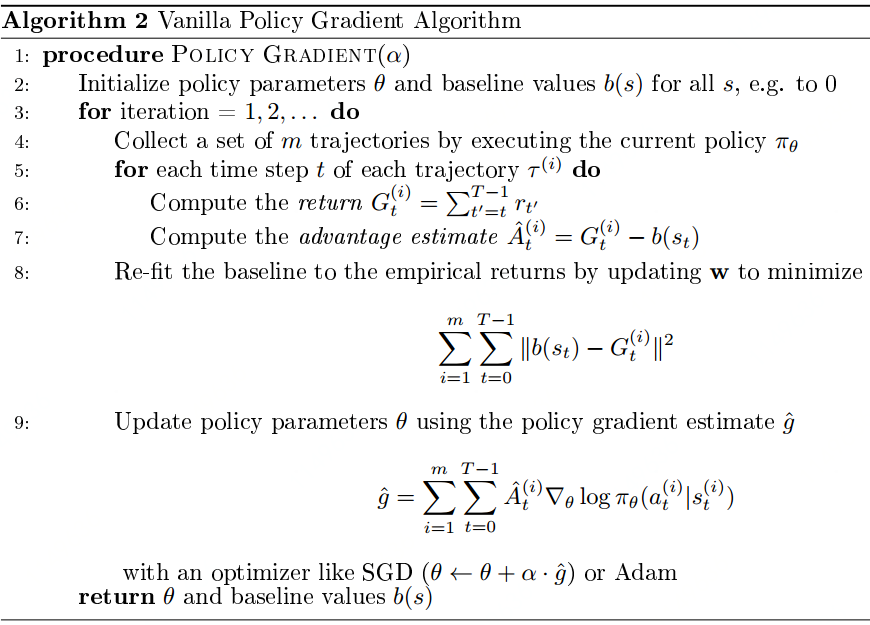 When considering the
  to be the value function
  . If we define the advantage function as
  , meanwhile, use an estimate
  as the true state values. The weight vector
  for the baseline (state-value) function and the policy parameters can be learned simultaneously using the Mote-Carlo trajectory samples.
Code implementation:
|
1 2 3 4 5 6 7 8 9 10 11 12 13 14 15 16 17 18 19 20 21 22 23 24 25 26 27 28 29 30 31 32 33 34 35 36 37 38 39 40 41 42 43 44 45 46 47 48 49 50 51 52 53 54 55 56 57 58 59 60 61 62 63 64 65 66 67 68 69 70 71 72 73 74 75 76 77 78 79 80 81 82 83 84 85 86 87 88 89 90 91 92 93 94 95 96 97 98 99 100 101 102 103 104 105 106 107 108 109 110 111 112 113 114 115 116 117 118 119 120 121 122 123 124 125 126 127 128 129 130 131 132 133 134 135 136 137 138 139 140 141 142 143 144 145 146 147 148 149 150 151 152 153 154 155 156 157 158 159 160 161 162 163 164 165 166 167 168 169 170 171 172 173 174 175 176 177 178 179 180 181 182 183 184 185 186 187 188 189 190 191 192 193 194 195 196 197 198 199 200 201 202 203 204 205 206 207 208 209 210 211 212 213 214 215 216 217 218 219 220 221 222 223 224 225 226 227 228 229 230 231 232 233 234 235 236 237 238 239 240 241 242 243 244 245 246 247 248 249 250 251 252 253 254 255 256 257 258 259 260 261 262 263 264 265 266 267 268 269 270 271 272 273 274 |
import numpy as np import tensorflow as tf import gym import time import scipy.signal from gym.spaces import Box, Discrete EPS = 1e-8 def combined_shape(length, shape=None): """ print(combined_shape(2)) #shape: (2,) print(combined_shape(2, shape=2)) #shape: (2, 2) print(combined_shape(None, 2)) #shape: (None, 2) print(combined_shape(None, None)) #shape: (None,) print(combined_shape(None, (2,3))) #shape: (None, 2, 3) print(combined_shape(2, shape=(2,3))) #shape: (2, 2, 3) print(combined_shape(2, shape=[2,3])) #shape: (2, 2, 3) print(combined_shape(2, shape={2,3})) #shape: (2, 2, 3) """ if shape is None: return (length, ) return (length, shape) if np.isscalar(shape) else (length, *shape) def placeholder(dim=None): return tf.placeholder(dtype=tf.float32, shape=combined_shape(None, dim)) def placeholders(*args): return [placeholder(dim) for dim in args] def placeholder_from_space(space): if isinstance(space, Box): return placeholder(space.shape) elif isinstance(space, Discrete): return tf.placeholder(dtype=tf.int32, shape=(None, )) raise NotImplementedError def placeholder_from_spaces(*args): return [placeholder_from_space(space) for space in args] def mlp(x, hidden_sizes=(32,), activation=tf.tanh, output_activaiton=None): for h in hidden_sizes[:-1]: #NULL, Escape x = tf.layers.dense(x, units=h, activation=activation) return tf.layers.dense(x, units=hidden_sizes[-1], activation=output_activaiton) #last layer def discount_cumsum(x, discount): """ input: vector x, [x0, x1, x2] output: [x0 + discount*x1 + discount^2*x2, x1 + discount*x2, x2] """ return scipy.signal.lfilter([1], [1, float(-discount)], x[::-1], axis=0)[::-1] def mlp_categorical_policy(x, a, hidden_sizes, activation, output_activation, action_space): act_dim = action_space.n # Add one more layer, raw prediciton layer, without nomalization logits = mlp(x, list(hidden_sizes)+[act_dim], activation, None) logp_all = tf.nn.log_softmax(logits) #Add softmax layer, --> [0,1] # tf.multinomial is a shorthand for tf.random.multinomial which just draws samples from a # multinomial distribution (which are unnormalized log probabilities in this case) pi = tf.squeeze(tf.multinomial(logits,1), axis=1) logp = tf.reduce_sum(tf.one_hot(a, depth=act_dim) * logp_all, axis=1) logp_pi = tf.reduce_sum(tf.one_hot(pi, depth=act_dim) * logp_all, axis=1) return pi, logp, logp_pi def guassian_likelihood(x, mu, log_std): pre_sum = -0.5 * ((x-mu)/(tf.exp(log_std)+EPS))**2 + 2*log_std + np.log(2*np.pi) return tf.reduce_sum(pre_sum, axis=1) def mlp_gaussian_policy(x, a, hidden_sizes, activation, output_actviation, action_space): act_dim = a.shape.as_list()[-1] mu = mlp(x, list(hidden_sizes)+[act_dim], activation, output_actviation) log_std = tf.get_variable(name='log_std', initializer=-0.5*np.ones(act_dim, dtype=np.float32)) std = tf.exp(log_std) pi = mu + tf.random_normal(tf.shape(mu)) * std logp = guassian_likelihood(a, mu, log_std) logp_pi = guassian_likelihood(pi, mu, log_std) return pi, logp, logp_pi def mlp_actor_critic(x, a, hidden_sizes=(64,64), activation=tf.tanh, output_activation=None, policy=None, action_space=None): if policy is None and isinstance(action_space, Box): policy = mlp_gaussian_policy elif policy is None and isinstance(action_space, Discrete): policy = mlp_categorical_policy with tf.variable_scope('pi'): pi, logp, logp_pi = policy(x, a, hidden_sizes, activation, output_activation, action_space) with tf.variable_scope('v'): v = tf.squeeze(mlp(x, list(hidden_sizes)+[1], activation, None), axis=1) return pi, logp, logp_pi, v def statistics_scalar(x, with_min_and_max=False): x = np.array(x, dtype=np.float32) x_sum, x_n = [np.sum(x), len(x)] mean = x_sum / x_n x_sum_sq = np.sum((x-mean)**2) std = np.sqrt(x_sum_sq/x_n) if with_min_and_max: x_min = np.min(x) if len(x)>0 else np.inf x_max = np.max(x) if len(x)>0 else -np.inf return mean, std, x_min, x_max return mean, std class VPGBuffer(object): """ A buffer for storing trajectories experienced by a VPG agent interacting with the environment, and using Generalized Advantage Estimation (GAE-Lambda) for calculating the advantages of state-action pairs. """ def __init__(self, obs_dim, act_dim, size, gamma=0.99, lam=0.95): self.obs_buf = np.zeros(combined_shape(size, obs_dim), dtype=np.float32) self.act_buf = np.zeros(combined_shape(size, act_dim), dtype=np.float32) self.adv_buf = np.zeros(size, dtype=np.float32) self.rew_buf = np.zeros(size, dtype=np.float32) self.ret_buf = np.zeros(size, dtype=np.float32) self.val_buf = np.zeros(size, dtype=np.float32) self.logp_buf = np.zeros(size, dtype=np.float32) self.gamma, self.lam = gamma, lam self.ptr, self.path_start_idx, self.max_size = 0, 0, size def store(self, obs, act, rew, val, logp): """ Append one timestep of agent-environment interaction to the buffer. """ assert self.ptr<self.max_size self.obs_buf[self.ptr] = obs self.act_buf[self.ptr] = act self.rew_buf[self.ptr] = rew self.val_buf[self.ptr] = val self.logp_buf[self.ptr] = logp self.ptr += 1 def finish_path(self, last_val=0): path_slice = slice(self.path_start_idx, self.ptr) rews = np.append(self.rew_buf[path_slice], last_val) vals = np.append(self.val_buf[path_slice], last_val) # the next two lines implement GAE-Lambda advantage calculation deltas = rews[:-1] + self.gamma * vals[1:] - vals[:-1] self.adv_buf[path_slice] = discount_cumsum(deltas, self.gamma * self.lam) # the next line computes rewards-to-go, to be targets for the value function self.ret_buf[path_slice] = discount_cumsum(rews, self.gamma)[:-1] self.path_start_idx = self.ptr def get(self): assert self.ptr == self.max_size self.ptr, self.path_start_idx = 0, 0 adv_mean, adv_std = statistics_scalar(self.adv_buf) self.adv_buf = (self.adv_buf - adv_mean) / adv_std return [self.obs_buf, self.act_buf, self.adv_buf, self.ret_buf, self.logp_buf] def vpg(env_fn, actor_critic=mlp_actor_critic, ac_kwargs=dict(), gamma=0.99, steps_per_epoch=3000, pi_lr=3e-4, vf_lr=1e-3, lam=0.97, train_v_iters=80, max_ep_len=1000, epochs=200, seed=0): """ Args: env_fn: A function which creates a copy of the environment. The environment must satisfy the OpenAI Gym API. actor_critic: A function which takes in placeholder symbols for state, ``x_ph``, and action, ``a_ph``, and returns the main outputs from the agent's Tensorflow computation graph: =========== ================ ====================================== Symbol Shape Description =========== ================ ====================================== ``pi`` (batch, act_dim) | Samples actions from policy given states. ``logp`` (batch,) | Gives log probability, according to the policy, of taking | actions ``a_ph`` in states ``x_ph``. ``logp_pi`` (batch,) | Gives log probability, according to | the policy, of the action sampled by``pi``. ``v`` (batch,) | Gives the value estimate for states in ``x_ph``. (Critical: | make sure to flatten this!) =========== ================ ====================================== ac_kwargs: Any kwargs appropriate for the actor_critic function you provided to VPG. seed (int): Seed for random number generators. gamma (float): Discount factor. (Always between 0 and 1.) steps_per_epoch (int): Number of steps of interaction (state-action pairs) for the agent and the environment in each epoch. pi_lr (float): Learning rate for policy optimizer. vf_lr (float): Learning rate for value function optimizer. lam (float): Lambda for GAE-Lambda. (Always between 0 and 1, close to 1.) train_v_iters (int): Number of gradient descent steps to take on value function per epoch. max_ep_len (int): Maximum length of trajectory / episode / rollout. epochs (int): Number of epochs of interaction (equivalent to number of policy updates) to perform. """ env = env_fn obs_dim = env.observation_space.shape #CartPole-v1:(4,) act_dim = env.action_space.shape #CartPole-v1:() ac_kwargs['action_space'] = env.action_space print(type(env.observation_space)) #<class 'gym.spaces.box.Box'> print(env.observation_space) #Box(4,) print(type(env.action_space)) #<class 'gym.spaces.discrete.Discrete'> print(env.action_space) #Discrete(2) print(isinstance(env.action_space, Box)) #False # Inputs to computation graph x_ph, a_ph = placeholder_from_spaces(env.observation_space, env.action_space) # Main outputs from computation graph adv_ph, ret_ph, logp_old_ph = placeholders(None, None, None) # Need all placeholders in *this* order later (to zip with data from buffer) pi, logp, logp_pi, v = actor_critic(x_ph, a_ph, **ac_kwargs) # Need all placeholders in *this* order later (to zip with data from buffer) all_phs = [x_ph, a_ph, adv_ph, ret_ph, logp_old_ph] # Every step, get: action, value, and logprob get_action_ops = [pi, v, logp_pi] # Experience buffer local_steps_per_epoch = int(steps_per_epoch) buf = VPGBuffer(obs_dim, act_dim, local_steps_per_epoch, gamma, lam) # VPG objectives pi_loss = - tf.reduce_mean(logp * adv_ph) v_loss = tf.reduce_mean((ret_ph - v)**2) # Info (useful to watch during learning) approx_kl = tf.reduce_mean(logp_old_ph - logp) # a sample estimate for KL-divergence approx_ent = tf.reduce_mean(-logp) # a sample estimate for entropy # Optimizers train_pi = tf.train.AdamOptimizer(learning_rate=pi_lr).minimize(pi_loss) train_v = tf.train.AdamOptimizer(learning_rate=vf_lr).minimize(v_loss) sess = tf.Session() sess.run(tf.global_variables_initializer()) def update(): inputs = {k:v for k,v in zip(all_phs, buf.get())} pi_l_old, v_l_old, ent = sess.run([pi_loss, v_loss, approx_ent], feed_dict=inputs) # Policy gradient steps sess.run(train_pi, feed_dict=inputs) for _ in range(train_v_iters): sess.run(train_v, feed_dict=inputs) # Log changes from update pi_l_new, v_l_new, kl = sess.run([pi_loss, v_loss, approx_kl], feed_dict=inputs) start_time = time.time() o, r, d, ep_ret, ep_len = env.reset(), 0 , False, 0, 0 for epoch in range(epochs): for t in range(local_steps_per_epoch): a, v_t, logp_t = sess.run(get_action_ops, feed_dict={x_ph: o.reshape(1, -1)}) buf.store(o, a, r, v_t, logp_t) o, r, d, _ = env.step(a[0]) ep_ret += r ep_len += 1 terminal = d or (ep_len == max_ep_len) if terminal or (t==local_steps_per_epoch-1): if not(terminal): print("Warning: trajectory cut off by epoch at %d steps."%ep_len) last_val = r if d else sess.run(v, feed_dict={x_ph: o.reshape(1, -1)}) buf.finish_path(last_val) if terminal: pass print("Episode Return %f" % ep_ret) o, r, d, ep_ret, ep_len = env.reset(), 0, False, 0, 0 update() env = gym.make("CartPole-v1") vpg(env_fn=env) |
Compare with actor-critic methods, whether the value function is used for policy evaluation.
5. Summary
A single graph to summary basic policy gradient methods and their relations as follow: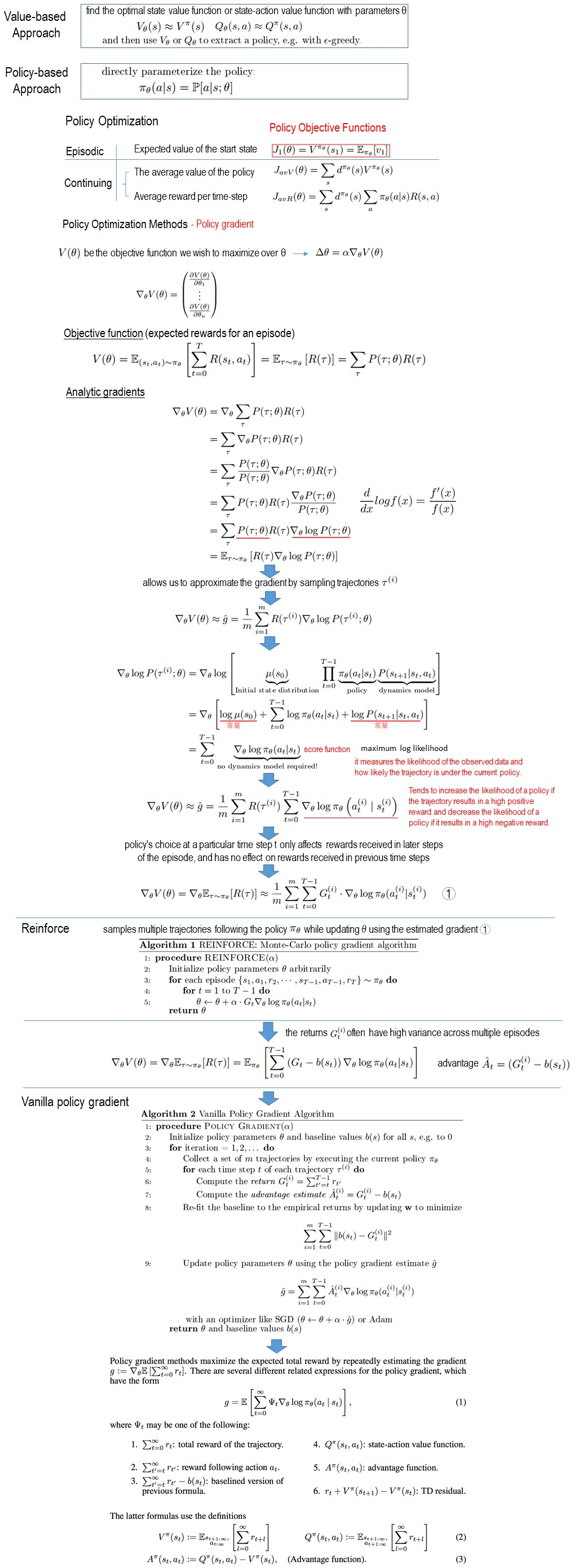
1 thought on “Policy Gradient Methods Overview”