In this post, we will start with a brief introduction of TD3 algorithm and why it is proposed, thus leading to the problem of overestimation bias and how it is handled in the actor-critic methods, together with some performance enhancement tricks by addressing variance. Furthermore, this post will also include two versions of state of art implementation to show its capability of promoting performance in continuous action space, one by OpenAI Spiningup, and the other from udemy. (Some of the post are selected directly from these reference to facilitate understanding)
This post is organized as follow:
1.Problem Formulation
2. Reducing Overestimation Bias
3. Addressing Variance
4. Psuedocode and Implementation
5. Reference
TD3 Overview
Twin Delayed Deep Deterministic Policy Gradient (TD3) is an off-policy algorithm that can only be used for environments with continuous action spaces, which gains improved performance over DDPG by introducing some critic tricks. The goal of TD3 algorithm is to solve the overestimation bias problem in actor-critic methods in continuous action spaces due to the function approximation error. In DDPG, a common failure mode is the learned Q-function begins to dramatically overestimate Q-values, which then leads to the policy breaking, because it exploits the errors in the Q-function.
1. Problem Formulation
The agent interacts with the environment at each discrete time step  , in the state
  , the agent selects actions
  according to its policy
  , receiving a scalar reward
  and the environment changes to the state
  . In this interaction process, return is defined as discounted sum of rewards from time after taking action
  in a state
  :
:
![\[{R_t} = \sum\nolimits_{i = t}^T {{\gamma ^{i - t}}r\left( {{s_i},{a_i}} \right)} \]](http://www.liaoyong.net/wp-content/ql-cache/quicklatex.com-9a59731110388e835d912615fc2c8140_l3.png "Rendered by QuickLaTeX.com")
 , with parameters
  , which maximizes the expected return
  :
: ![\[J\left( \phi \right) = {{\mathbb{E}}_{{s_i} \sim {p_{\rm{\pi }}},{a_i} \sim {\rm{\pi }}}}\left[ {{R_0}} \right]\]](http://www.liaoyong.net/wp-content/ql-cache/quicklatex.com-10eff286e4e65847667a6a0fa5df5ba9_l3.png "Rendered by QuickLaTeX.com")
 , namely,
 ![\[\max J\left(\phi \right) \]](http://www.liaoyong.net/wp-content/ql-cache/quicklatex.com-73c057ef889debe36697299dfd8d8e3e_l3.png "Rendered by QuickLaTeX.com")
is differential with respect to , using gradient ascent method, parameterized policies can be updated by taking the gradient of the expected return 
In the actor-critic setting, the policy, namely the actor, according to the deterministic policy gradient theorem (refer to DPG section), can be updated through:
![\[{\nabla _\phi }J\left( \phi \right){\rm{ = }}{{\mathbb{E}}_{s \sim {p_{\rm{\pi }}}}}\left[ {{\nabla _a}{Q^{\rm{\pi }}}\left( {s,a} \right)\left| {_{a = {\rm{\pi }}(s)}{\nabla _\phi }{{\rm{\pi }}_\phi }(s)} \right.} \right]\]](http://www.liaoyong.net/wp-content/ql-cache/quicklatex.com-33b0967812de3fb4a35e8f9912b931d3_l3.png "Rendered by QuickLaTeX.com")
 is the expected return when performing action in state and following
  after, is known as the critic or the value function, denoted as:
 ![\[{Q^{\rm{\pi }}}\left( {s,a} \right) = {{\mathbb{E}}_{{s_i} \sim {p_{\rm{\pi }}},{a_i} \sim {\rm{\pi }}}}\left[ {{R_t}\left| {s,a} \right.} \right]\]](http://www.liaoyong.net/wp-content/ql-cache/quicklatex.com-326fe3e76a6a9a22609eaa74e8ca2ac4_l3.png "Rendered by QuickLaTeX.com")
 , which may varies due to the cases of different sizes.
In small state space, using Q-learning,
 or the value function can be learned using temporal difference learning based on the Bellman equation, which is a fundamental relationship between the value of a state-action pair
  and the value of the subsequent state-action pair
  :
: ![\[{Q^{\rm{\pi }}}\left( {s,a} \right) = r + \gamma {{\mathbb{E}}_{s',a'}}\left[ {{Q^{\rm{\pi }}}\left( {s',a'} \right)} \right],\;{\kern 1pt} a \sim {\rm{\pi }}(s')\]](http://www.liaoyong.net/wp-content/ql-cache/quicklatex.com-0e2a99c36283d6c9a4cd37764a526236_l3.png "Rendered by QuickLaTeX.com")
 , with parameters
  , which is the neural network approximator in deep Q-learning , the network is updated by using temporal difference learning with a secondary frozen target network
  to maintain a fixed objective
  over multiple updates:
 ![\[y = r + \gamma {Q_{\theta '}}\left( {s',a'} \right),\;{\kern 1pt} a \sim {{\rm{\pi }}_{\phi '}}(s')\]](http://www.liaoyong.net/wp-content/ql-cache/quicklatex.com-14ec00cd62e85563629444022c8d2e02_l3.png "Rendered by QuickLaTeX.com")
 .
.The target network updates periodically to exactly match the weights of the current network, or by some proportion
 at each time step according to
  .
.By minimizing the difference between the action value and its target, or loss below, using the deep learning framework, we can finally get the parameters.
![\[Loss = {\left( {{Q^{\rm{\pi }}}\left( {s,a;\theta } \right) - y} \right)^2}\]](http://www.liaoyong.net/wp-content/ql-cache/quicklatex.com-ce1e58295c6e7d1cabd21ab242871f8e_l3.png "Rendered by QuickLaTeX.com")
2. Reducing Overestimation Bias
What’s overestimation bias?
(From TD3 paper) Overestimation bias is a property of Q-learning in which the maximization of a noisy value estimate induces a consistent overestimation. In a function approximation setting, this noise is unavoidable given the imprecision of the estimator. This inaccuracy is further exaggerated by the nature of temporal difference learning, in which an estimate of the value function is updated using the estimate of a subsequent state. This means using an imprecise estimate within each update will lead to an accumulation of error. Due to overestimation bias, this accumulated error can cause arbitrarily bad states to be estimated as high value, resulting in suboptimal policy updates and divergent behavior.
In Q-learning with discrete actions, the value estimate is updated with a greedy target  , when the
  is corrupted by errors due to the estimation error, the agent using the maximization operation may select a wrong action that causes a overestimation bias, and will be then propagated through the Bellman equation. The overestimation bias is obvious in the discrete action setting compared with the actor-critic setting where policy is updated via gradient descent. TD3 paper section 4.1 proves the overestimation bias also exists in actor-critic setting.
How to reduce the effects of overestimation bias?
For Q-learning, the Double Q-learning is proposed, its greedy update uses two independent estimators, each is used to update the other: (Double Q-learning setting)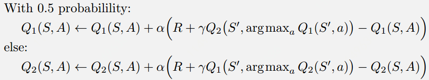 For DQN, the Double DQN is proposed to use the target network as one of the value estimates, and obtain a policy by greedy maximization of the current value network rather than the target network. (Double DQN setting)
![\[y_t^{{\rm{DoubleDQN}}} = {r_{t + 1}} + \gamma Q\left( {{s_{t + 1}},\arg {{\max }_a}Q\left( {{s_{t + 1}},a;{\theta _t}} \right),\theta _t^ - } \right)\]](http://www.liaoyong.net/wp-content/ql-cache/quicklatex.com-583e05795a3db1e5f8ea2223617a8ff6_l3.png "Rendered by QuickLaTeX.com")
![\[y = r + \gamma {Q_{\theta '}}\left( {s',{{\rm{\pi }}_\phi }(s')} \right)\]](http://www.liaoyong.net/wp-content/ql-cache/quicklatex.com-0053fe2dad3b9cf485eaa0bc7fae6498_l3.png "Rendered by QuickLaTeX.com")
 and critics
  , where
  is optimized with respected to
  and
and  with respected to
  : (Actor-critic Double DQN setting)
 ![\[\begin{array}{l}{y_1} = r + \gamma {Q_{{{\theta '}_2}}}\left( {s',{{\rm{\pi }}_{{\phi _1}}}(s')} \right)\\{y_2} = r + \gamma {Q_{{{\theta '}_1}}}\left( {s',{{\rm{\pi }}_{{\phi _2}}}(s')} \right)\end{array}\]](http://www.liaoyong.net/wp-content/ql-cache/quicklatex.com-e0a7522e42dcb3d394bd00cf4e6f9eab_l3.png "Rendered by QuickLaTeX.com")
and , the target is updated by: ![\[{y_1} = r + \gamma \mathop {\min }\limits_{i = 1,2} {Q_{{{\theta '}_i}}}\left( {s',{{\rm{\pi }}_{{\phi _1}}}(s')} \right)\]](http://www.liaoyong.net/wp-content/ql-cache/quicklatex.com-9606da12e9ac463ba92352a58cc9d731_l3.png "Rendered by QuickLaTeX.com")
To get an overview of how this Clipped Double Q-learning target update rule is formed? The original TD3 paper explores in the following procedure:
 Takeaway: TD3 uses the Double Q-learning ways, it learns two Q-functions instead of one (hence “twin”), and uses the smaller of the two Q-values to form the targets in the Bellman error loss functions.
3. Addressing Variance
Three approaches are proposed to addressing the variance directly, namely, using target network, delayed policy update and a regularization strategy.
(1)Target Networks and Delayed Policy Update
The paper proves using a stable target reduces the growth of error and shows divergence will occur without target networks is the result of policy updates with a high variance value estimate. Value estimates diverge through overestimation when the policy is poor, and the policy will become poor if the value estimate itself is inaccurate.
(From TD3 paper) If target networks can be used to reduce the error over multiple updates, and policy updates on high-error states cause divergent behavior, then the policy network should be updated at a lower frequency than the value network, to first minimize error before introducing a policy update. We propose delaying policy updates until the value error is as small as possible. The target networks are updated slowly by:
![\[\theta ' \leftarrow \tau \theta + (1 - \tau )\theta '\]](http://www.liaoyong.net/wp-content/ql-cache/quicklatex.com-6707207967752bbbb0159a6cfc673123_l3.png "Rendered by QuickLaTeX.com")
The deterministic policies can overfit to narrow peaks in the value estimate, a common sense is that similar actions should have similar value. Fit the value of a small area around the target action:
![\[y = r + {\mathbb{E}_\epsilon }\left[ {{Q_{\theta '}}\left( {s',{{\rm{\pi }}_{\phi '}}(s') + \epsilon } \right)} \right]\]](http://www.liaoyong.net/wp-content/ql-cache/quicklatex.com-7a4a5e558eab9864d3bf12042efd8943_l3.png "Rendered by QuickLaTeX.com")
![\[\begin{array}{l}y = r + \gamma {Q_{\theta '}}\left( {s',{{\rm{\pi }}_{\phi '}}(s') + \epsilon } \right),\\\epsilon \sim clip\left( {N(0,\sigma ), - c,c} \right)\end{array}\]](http://www.liaoyong.net/wp-content/ql-cache/quicklatex.com-8dcc62612e4795b606f886a67e8e83c3_l3.png "Rendered by QuickLaTeX.com")
Takeaway: TD3 updates the policy (and target networks) less frequently than the Q-function. It adds noise to the target action, to make it harder for the policy to exploit Q-function errors by smoothing out Q along changes in action.
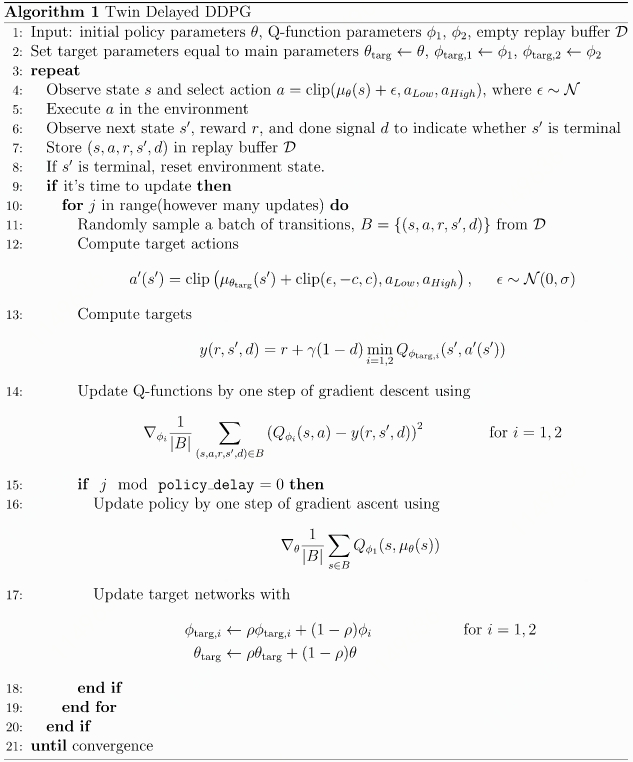
4. Pseudocode and Implementation
Version1: Main process of learning(Selected and summarized from OpenAI Spinning Up explanation).
Step1: Taking Action (do target policy smoothing), get  .
.
Actions used to form the Q-learning target are based on the target policy  , but with clipped noise added on each dimension of the action. After adding the clipped noise, the target action is then clipped to lie in the valid action range (all valid actions, , satisfy
  . The target actions are thus:
![\[a'(s') = {\rm{clip}}\left( {{\mu _{{\theta _{{\rm{targ}}}}}}\left( {s'} \right) + {\rm{clip}}\left( {\varepsilon , - c,c} \right),{a_{Low}},{a_{High}}} \right),\;\;\varepsilon \sim \;N(0,\sigma )\]](http://www.liaoyong.net/wp-content/ql-cache/quicklatex.com-1f6d8357e04c3085a1a10d2610e62617_l3.png "Rendered by QuickLaTeX.com")
Both Q-functions use a single target, calculated using whichever of the two Q-functions gives a smaller target value:
![\[y(r,s',d) = r + \gamma (1 - d)\mathop {\min }\limits_{i = 1,2} {Q_{{\theta _{i,{\rm{targ}}}}}}\left( {s',a'(s')} \right),\]](http://www.liaoyong.net/wp-content/ql-cache/quicklatex.com-a83676e50afe5a9cdf18d213de1a8664_l3.png "Rendered by QuickLaTeX.com")
![\[\begin{array}{l}L\left( {{\phi _1},D} \right) = \mathop \mathbb{E}\limits_{(s,a,r,s',d) \sim D} \left[ {{{\left( {{Q_{{\phi _1}}}\left( {s,a} \right) - y(r,s',d)} \right)}^2}} \right]\\L\left( {{\phi _2},D} \right) = \mathop \mathbb{E}\limits_{(s,a,r,s',d) \sim D} \left[ {{{\left( {{Q_{{\phi _2}}}\left( {s,a} \right) - y(r,s',d)} \right)}^2}} \right]\end{array}\]](http://www.liaoyong.net/wp-content/ql-cache/quicklatex.com-8393796b87097601d2a6f3702dd869af_l3.png "Rendered by QuickLaTeX.com")
Step3: Policy learning
The policy is learned just by maximizing

![\[\mathop {\max }\limits_\theta \mathop \mathbb{E}\limits_{s \sim D} \left[ {{Q_{{\phi _1}}}\left( {s,{\mu _\theta }(s)} \right)} \right]\]](http://www.liaoyong.net/wp-content/ql-cache/quicklatex.com-4e80f6ae03985a433a31a2923a86a213_l3.png "Rendered by QuickLaTeX.com")
 The following code implementation is modified from original OpenAI Spinninng-up Github to make it is much easier to understand just in one single file:
Implemntation Version1:
|
1 2 3 4 5 6 7 8 9 10 11 12 13 14 15 16 17 18 19 20 21 22 23 24 25 26 27 28 29 30 31 32 33 34 35 36 37 38 39 40 41 42 43 44 45 46 47 48 49 50 51 52 53 54 55 56 57 58 59 60 61 62 63 64 65 66 67 68 69 70 71 72 73 74 75 76 77 78 79 80 81 82 83 84 85 86 87 88 89 90 91 92 93 94 95 96 97 98 99 100 101 102 103 104 105 106 107 108 109 110 111 112 113 114 115 116 117 118 119 120 121 122 123 124 125 126 127 128 129 130 131 132 133 134 135 136 137 138 139 140 141 142 143 144 145 146 147 148 149 150 151 152 153 154 155 156 157 158 159 160 161 162 163 164 165 166 167 168 169 170 171 172 173 174 175 176 177 178 179 180 181 182 183 184 185 186 187 188 189 190 191 192 193 194 195 196 197 198 199 200 201 202 203 204 205 206 207 208 209 210 211 212 213 214 215 216 217 218 219 220 221 222 223 224 225 226 227 228 229 230 231 232 233 234 235 236 237 238 239 240 241 242 243 244 245 246 247 248 249 250 251 252 253 254 255 256 257 258 259 260 261 262 263 264 265 266 267 268 269 270 271 272 273 274 275 276 277 278 |
import numpy as np import tensorflow as tf import gym def placeholder(dim=None): return tf.placeholder(dtype=tf.float32, shape=(None, dim) if dim else (None,)) def placeholders(*args): return [placeholder(dim) for dim in args] def mlp(x, hidden_sizes=(32,), activation=tf.tanh, output_activation=None): for h in hidden_sizes[:-1]: x = tf.layers.dense(x, units=h, activation=activation) return tf.layers.dense(x, hidden_sizes[-1], activation=output_activation) def get_vars(scope): return [x for x in tf.global_variables() if scope in x.name] def count_vars(scope): v = get_vars(scope) return sum([np.prod(var.shape.as_list()) for var in v]) # Actor-Critic def mlp_actor_critic(x, a, hidden_sizes=(256,256), activation=tf.nn.relu, output_activation=tf.tanh, action_space=None): act_dim = a.shape.as_list()[-1] act_limit = action_space.high[0] with tf.variable_scope('pi'): pi = act_limit * mlp(x, list(hidden_sizes)+[act_dim], activation, output_activation) with tf.variable_scope('q1'): q1 = tf.squeeze(mlp(tf.concat([x,a], axis=-1), list(hidden_sizes)+[1], activation, None), axis=1) with tf.variable_scope('q2'): q2 = tf.squeeze(mlp(tf.concat([x,a], axis=-1), list(hidden_sizes)+[1], activation, None), axis=1) with tf.variable_scope('q1', reuse=True): q1_pi = tf.squeeze(mlp(tf.concat([x,pi], axis=-1), list(hidden_sizes)+[1], activation, None), axis=1) return pi, q1, q2, q1_pi class ReplayBuffer(object): """A simple FIFO experience replay buffer for TD3 agents.""" def __init__(self, obs_dim, act_dim, size): self.obs1_buf = np.zeros([size, obs_dim], dtype=np.float32) self.obs2_buf = np.zeros([size, obs_dim], dtype=np.float32) self.acts_buf = np.zeros([size, act_dim], dtype=np.float32) self.rews_buf = np.zeros(size, dtype=np.float32) self.done_buf = np.zeros(size, dtype=np.float32) self.ptr, self.size, self.max_size = 0, 0, size def store(self, obs, act, rew, next_obs, done): self.obs1_buf[self.ptr] = obs self.obs2_buf[self.ptr] = next_obs self.acts_buf[self.ptr] = act self.rews_buf[self.ptr] = rew self.done_buf[self.ptr] = done self.ptr = (self.ptr+1) % self.max_size self.size = min(self.size+1, self.max_size) def sample_batch(self, batch_size=32): idxs = np.random.randint(0, self.size, size=batch_size) return dict(obs1=self.obs1_buf[idxs], obs2=self.obs2_buf[idxs], acts=self.acts_buf[idxs], rews=self.rews_buf[idxs], done=self.done_buf[idxs]) def td3(env_fn, actor_critic=mlp_actor_critic, ac_kwargs=dict(), seed=0, steps_per_epoch=4000, epochs=100, replay_size=int(1e6), gamma=0.99, polyak=0.995, pi_lr=1e-3, q_lr=1e-3, batch_size=100, start_steps=10000, update_after=1000, update_every=50, act_noise=0.1, target_noise=0.2, noise_clip=0.5, policy_delay=2, num_test_episodes=10, max_ep_len=1000): """ Twin Delayed Deep Deterministic Policy Gradient (TD3) Args: env_fn : A function which creates a copy of the environment. The environment must satisfy the OpenAI Gym API. actor_critic: A function which takes in placeholder symbols for state, ``x_ph``, and action, ``a_ph``, and returns the main outputs from the agent's Tensorflow computation graph: =========== ================ ====================================== Symbol Shape Description =========== ================ ====================================== ``pi`` (batch, act_dim) | Deterministically computes actions | from policy given states. ``q1`` (batch,) | Gives one estimate of Q* for | states in ``x_ph`` and actions in | ``a_ph``. ``q2`` (batch,) | Gives another estimate of Q* for | states in ``x_ph`` and actions in | ``a_ph``. ``q1_pi`` (batch,) | Gives the composition of ``q1`` and | ``pi`` for states in ``x_ph``: | q1(x, pi(x)). =========== ================ ====================================== ac_kwargs (dict): Any kwargs appropriate for the actor_critic function you provided to TD3. seed (int): Seed for random number generators. steps_per_epoch (int): Number of steps of interaction (state-action pairs) for the agent and the environment in each epoch. epochs (int): Number of epochs to run and train agent. replay_size (int): Maximum length of replay buffer. gamma (float):<span style="background-color: #ff6600;"> Discount factor</span>. (Always between 0 and 1.) polyak (float): Interpolation factor in polyak averaging for target networks. Target networks are updated towards main networks according to: .. math:: \\theta_{\\text{targ}} \\leftarrow \\rho \\theta_{\\text{targ}} + (1-\\rho) \\theta where :math:`\\rho` is polyak. (Always between 0 and 1, usually close to 1.) pi_lr (float): Learning rate for policy. q_lr (float): Learning rate for Q-networks. batch_size (int): Minibatch size for SGD. start_steps (int): Number of steps for uniform-random action selection, before running real policy. Helps exploration. update_after (int): Number of env interactions to collect before starting to do gradient descent updates. Ensures replay buffer is full enough for useful updates. update_every (int): Number of env interactions that should elapse between gradient descent updates. Note: Regardless of how long you wait between updates, the ratio of env steps to gradient steps is locked to 1. act_noise (float): Stddev for Gaussian exploration noise added to policy at training time. (At test time, no noise is added.) target_noise (float): Stddev for smoothing noise added to target policy. noise_clip (float): Limit for absolute value of target policy smoothing noise. policy_delay (int): Policy will only be updated once every policy_delay times for each update of the Q-networks. num_test_episodes (int): Number of episodes to test the deterministic policy at the end of each epoch. max_ep_len (int): Maximum length of trajectory / episode / rollout. logger_kwargs (dict): Keyword args for EpochLogger. save_freq (int): How often (in terms of gap between epochs) to save the current policy and value function. """ tf.set_random_seed(seed) np.random.seed(seed) env, test_env = env_fn(), env_fn() obs_dim = env.observation_space.shape[0] act_dim = env.action_space.shape[0] # Action limit for clamping: critically, assumes all dimensions share the same bound! act_limit = env.action_space.high[0] # Share information about action space with policy architecture ac_kwargs['action_space'] = env.action_space # Inputs to computation graph x_ph, a_ph, x2_ph, r_ph, d_ph = placeholders(obs_dim, act_dim, obs_dim, None, None) # Main outputs from computation graph with tf.variable_scope('main'): pi, q1, q2, q1_pi = actor_critic(x_ph, a_ph, **ac_kwargs) # Target policy network with tf.variable_scope('target'): pi_targ, _, _, _ = actor_critic(x2_ph, a_ph, **ac_kwargs) # Target Q networks with tf.variable_scope('target', reuse=True): # Target policy smoothing, by adding clipped noise to target actions epsilon = tf.random_normal(tf.shape(pi_targ), stddev=target_noise) epsilon = tf.clip_by_value(epsilon, -noise_clip, noise_clip) a2 = pi_targ + epsilon a2 = tf.clip_by_value(a2, -act_limit, act_limit) # Target Q-values, using action from target policy _, q1_targ, q2_targ, _ = actor_critic(x2_ph, a2, **ac_kwargs) # Experience buffer replay_buffer = ReplayBuffer(obs_dim=obs_dim, act_dim=act_dim, size=replay_size) # Count variables var_counts = tuple(count_vars(scope) for scope in ['main/pi', 'main/q1', 'main/q2', 'main']) print('\nNumber of parameters: \t pi: %d, \t q1: %d, \t q2: %d, \t total: %d'%var_counts) # Bellman backup for Q functions, using Clipped Double-Q target min_q_targ = tf.minimum(q1_targ, q2_targ) backup = tf.stop_gradient(r_ph + gamma*(1-d_ph)*min_q_targ) # TD3 losses pi_loss = -tf.reduce_mean(q1_pi) q1_loss = tf.reduce_mean((q1-backup)**2) q2_loss = tf.reduce_mean((q2-backup)**2) q_loss = q1_loss + q2_loss # Separate train ops for pi, q pi_optimizer = tf.train.AdamOptimizer(learning_rate=pi_lr) q_optimizer = tf.train.AdamOptimizer(learning_rate=q_lr) train_pi_op = pi_optimizer.minimize(pi_loss, var_list=get_vars('main/pi')) train_q_op = q_optimizer.minimize(q_loss, var_list=get_vars('main/q')) # Polyak averaging for target variables target_update = tf.group([tf.assign(v_targ, polyak*v_targ + (1-polyak)*v_main) for v_main, v_targ in zip(get_vars('main'), get_vars('target'))]) # Initializing targets to match main variables target_init = tf.group([tf.assign(v_targ, v_main) for v_main, v_targ in zip(get_vars('main'), get_vars('target'))]) sess = tf.Session() sess.run(tf.global_variables_initializer()) sess.run(target_init) def get_action(o, noise_scale): a = sess.run(pi, feed_dict={x_ph: o.reshape(1,-1)})[0] a += noise_scale * np.random.rand(act_dim) return np.clip(a, -act_limit, act_limit) def test_agent(): for j in range(num_test_episodes): o, d, ep_ret, ep_len = test_env.reset(), False, 0, 0 while not(d or (ep_len==max_ep_len)): # Take deterministic actions at test time (noise_scale=0) o, r, d, _ = test_env.step(get_action(o, 0)) ep_ret += r ep_len += 1 print('# TestEpRet={}, TestEpLen={}'.format(ep_ret, ep_len)) o, ep_ret, ep_len = env.reset(), 0, 0 total_steps = steps_per_epoch * epochs # Main loop: collect experience in env and update/log each epoch for t in range(total_steps): # Until start_steps have elapsed, randomly sample actions # from a uniform distribution for better exploration. Afterwards, # use the learned policy (with some noise, via act_noise). if t > start_steps: a = get_action(o, act_noise) else: a = env.action_space.sample() # Step the env o2, r, d, _ = env.step(a) ep_ret += r ep_len += 1 # Ignore the "done" signal if it comes from hitting the time horizon (that is, when it's an # artificial terminal signal that isn't based on the agent's state) d = False if ep_len==max_ep_len else d # Store experience to replay buffer replay_buffer.store(o, a, r, o2, d) # Super critical, easy to overlook step: make sure to update most recent observation! o = o2 # End of trajectory handling if d or (ep_len == max_ep_len): print('EpRet={}, EpLen={}'.format(ep_ret, ep_len)) o, ep_ret, ep_len = env.reset(), 0, 0 # Update handling if t>=update_after and t%update_every==0: for j in range(update_every): batch = replay_buffer.sample_batch(batch_size) feed_dict = {x_ph: batch['obs1'], x2_ph: batch['obs2'], a_ph: batch['acts'], r_ph: batch['rews'], d_ph: batch['done']} q_step_ops = [q_loss, q1, q2, train_q_op] outs = sess.run(q_step_ops, feed_dict) # print('#LossQ={}, Q1Vals={}, Q2Vals={}'.format(outs[0], outs[1], outs[2])) if j % policy_delay == 0: # Delayed policy update outs = sess.run([pi_loss, train_pi_op, target_update], feed_dict) # print('#LossPi={}'.format(outs[0])) # End of epoch wrap-up if (t+1) % steps_per_epoch == 0: test_agent() if __name__ == '__main__': env = 'MountainCarContinuous-v0' hid = 256 l = 2 gamma = 0.99 seed = 0 epochs = 50 exp_name = 'td3' td3(lambda : gym.make(env), actor_critic=mlp_actor_critic, ac_kwargs=dict(hidden_sizes=[hid]*l), gamma=gamma, seed=seed, epochs=epochs) |
The results of is as follow: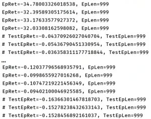
Version2:
This section we will the other version of implementation, modified from udemy reinforcement learning 2.0, following the original TD3 paper. Coresponding pseudocdoe is shown as follow:
Procedure of implementing this algorithm according to the original paper:
Initialization
Step1: Initialize the experience replay memory, with a size of 20000 and it will be populated with each new transition.
Step2: Build one neural network for the actor model and one neural network for the actor target.
Step3: Build two neural networks for the two critic models and two neural networks for the two critic targets.
Training Process – run a full episode with first 10000 actions played randomly, and with actions played by the actor model. Then repeat the following steps:
Step4: Sample a batch of transitions  from the memory. Then for each element of the batch:
Step5: From the next state  , the actor target plays the next action
  .
.
Step6: Add the Gaussian noise to this next action and clamp it in a range of values supported by the environment.
Step7: The two critic targets take each the couple  as input and return two Q-values,
  and
and  as outputs.
Step8: Keep the minimum of these two Q-values: . It represents the approximated value of the next state.
Step9: Get the final target of the two critic models, which is:  , where
  is the discount factor.
Step10: The two critic models take each the couple  ) as input and return two Q-values
  and
and  as outputs.
Step11: Compute the loss coming from the two critic models: 
Step12: Backpropagate this Critic Loss and update the parameters of the two critic models with a SGD optimizer.
Step13: Once every two iterations, update the actor model by performing gradient ascent on the output the first critic model:
![\[{\nabla _\phi }J\left( \phi \right){\rm{ = }}{N^{ - 1}}\sum {{\nabla _a}{Q_{{\theta _1}}}\left( {s,a} \right)\left| {_{a = {{\rm{\pi }}_\phi }(s)}{\nabla _\phi }{{\rm{\pi }}_\phi }(s)} \right.} \]](http://www.liaoyong.net/wp-content/ql-cache/quicklatex.com-0ee068a0bc335be952de01cb541dd91a_l3.png "Rendered by QuickLaTeX.com")
and  represent the weights of the actor and critic.
Step14: Still once two iterations, update the weights of the actor target by polyak averaging:
![\[{{\theta '}_i} \leftarrow \tau {\theta _i} + (1 - \tau ){{\theta '}_i}\]](http://www.liaoyong.net/wp-content/ql-cache/quicklatex.com-4d32c23d9017fd1b4e139bdb4436fabd_l3.png "Rendered by QuickLaTeX.com")
![\[\phi ' \leftarrow \tau \phi + (1 - \tau )\phi '\]](http://www.liaoyong.net/wp-content/ql-cache/quicklatex.com-6e6857954a7d5a195e3341e783c49789_l3.png "Rendered by QuickLaTeX.com")
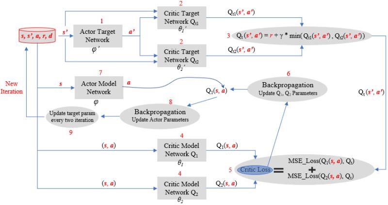 We can aslo refer to the original diagram (from reference 3) introduced as bellow for understanding.
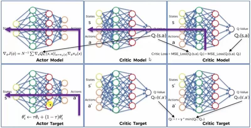
Version 2:
The Full code implementation is as follow, three enviroments are test in this code, all of them work perfect well.
|
1 2 3 4 5 6 7 8 9 10 11 12 13 14 15 16 17 18 19 20 21 22 23 24 25 26 27 28 29 30 31 32 33 34 35 36 37 38 39 40 41 42 43 44 45 46 47 48 49 50 51 52 53 54 55 56 57 58 59 60 61 62 63 64 65 66 67 68 69 70 71 72 73 74 75 76 77 78 79 80 81 82 83 84 85 86 87 88 89 90 91 92 93 94 95 96 97 98 99 100 101 102 103 104 105 106 107 108 109 110 111 112 113 114 115 116 117 118 119 120 121 122 123 124 125 126 127 128 129 130 131 132 133 134 135 136 137 138 139 140 141 142 143 144 145 146 147 148 149 150 151 152 153 154 155 156 157 158 159 160 161 162 163 164 165 166 167 168 169 170 171 172 173 174 175 176 177 178 179 180 181 182 183 184 185 186 187 188 189 190 191 192 193 194 195 196 197 198 199 200 201 202 203 204 205 206 207 208 209 210 211 212 213 214 215 216 217 218 219 220 221 222 223 224 225 226 227 228 229 230 231 232 233 234 235 236 237 238 239 240 241 242 243 244 245 246 247 248 249 250 251 252 253 254 255 256 257 258 259 260 261 262 263 264 265 266 267 268 269 270 271 272 273 274 275 276 277 278 279 280 281 282 283 284 285 286 287 288 289 290 291 292 293 294 295 296 297 298 299 300 301 302 303 304 305 306 307 308 309 310 311 312 313 314 315 316 317 318 319 320 321 322 323 324 325 326 327 328 329 330 331 332 333 334 335 336 337 338 |
import os import time import random import numpy as np import matplotlib.pyplot as plt import pybullet_envs import gym import torch import torch.nn as nn import torch.nn.functional as F from gym import wrappers from torch.autograd import Variable from collections import deque # Step 1: Initialize the Experience Replay memory class ReplayBuffer(object): def __init__(self, max_size=1e6): self.storage = [] self.max_size = max_size self.ptr = 0 def add(self, transition): if len(self.storage) == self.max_size: self.storage[int(self.ptr)] = transition self.ptr = (self.ptr + 1) % self.max_size else: self.storage.append(transition) def sample(self, batch_size): ind = np.random.randint(0, len(self.storage), size=batch_size) batch_states, batch_next_states, batch_actions, batch_rewards, batch_dones = [], [], [], [], [] for i in ind: state, next_state, action, reward, done = self.storage[i] batch_states.append(np.array(state, copy=False)) batch_next_states.append(np.array(next_state, copy=False)) batch_actions.append(np.array(action, copy=False)) batch_rewards.append(np.array(reward, copy=False)) batch_dones.append(np.array(done, copy=False)) return np.array(batch_states), np.array(batch_next_states), np.array(batch_actions), np.array( batch_rewards).reshape(-1, 1), np.array(batch_dones).reshape(-1, 1) # Build one neural network for the Actor model and one neural network for the Actor target class Actor(nn.Module): def __init__(self, state_dim, action_dim, max_action): super(Actor, self).__init__() self.layer_1 = nn.Linear(state_dim, 400) self.layer_2 = nn.Linear(400, 300) self.layer_3 = nn.Linear(300, action_dim) self.max_action = max_action def forward(self, x): x = F.relu(self.layer_1(x)) x = F.relu(self.layer_2(x)) x = self.max_action * torch.tanh(self.layer_3(x)) return x # Build two neural networks for the two Critic models and two neural networks for the two Critic targets class Critic(nn.Module): def __init__(self, state_dim, action_dim): super(Critic, self).__init__() # Defining the first Critic neural network self.layer_1 = nn.Linear(state_dim + action_dim, 400) self.layer_2 = nn.Linear(400, 300) self.layer_3 = nn.Linear(300, 1) # Defining the second Critic neural network self.layer_4 = nn.Linear(state_dim + action_dim, 400) self.layer_5 = nn.Linear(400, 300) self.layer_6 = nn.Linear(300, 1) def forward(self, x, u): xu = torch.cat([x, u], 1) # Forward-Propagation on the first Critic Neural Network x1 = F.relu(self.layer_1(xu)) x1 = F.relu(self.layer_2(x1)) x1 = self.layer_3(x1) # Forward-Propagation on the second Critic Neural Network x2 = F.relu(self.layer_4(xu)) x2 = F.relu(self.layer_5(x2)) x2 = self.layer_6(x2) return x1, x2 def Q1(self, x, u): xu = torch.cat([x, u], 1) x1 = F.relu(self.layer_1(xu)) x1 = F.relu(self.layer_2(x1)) x1 = self.layer_3(x1) return x1 ## Training Process # Selecting the device (CPU or GPU) device = torch.device("cuda" if torch.cuda.is_available() else "cpu") # Building the whole Training Process into a class class TD3(object): def __init__(self, state_dim, action_dim, max_action): self.actor = Actor(state_dim, action_dim, max_action).to(device) self.actor_target = Actor(state_dim, action_dim, max_action).to(device) self.actor_target.load_state_dict(self.actor.state_dict()) self.actor_optimizer = torch.optim.Adam(self.actor.parameters()) self.critic = Critic(state_dim, action_dim).to(device) self.critic_target = Critic(state_dim, action_dim).to(device) self.critic_target.load_state_dict(self.critic.state_dict()) self.critic_optimizer = torch.optim.Adam(self.critic.parameters()) self.max_action = max_action def select_action(self, state): state = torch.Tensor(state.reshape(1, -1)).to(device) return self.actor(state).cpu().data.numpy().flatten() def train(self, replay_buffer, iterations, batch_size=100, discount=0.99, tau=0.005, policy_noise=0.2, noise_clip=0.5, policy_freq=2): for it in range(iterations): # Step 4: Sample a batch of transitions (s, s’, a, r) from the memory batch_states, batch_next_states, batch_actions, batch_rewards, batch_dones = replay_buffer.sample( batch_size) state = torch.Tensor(batch_states).to(device) next_state = torch.Tensor(batch_next_states).to(device) action = torch.Tensor(batch_actions).to(device) reward = torch.Tensor(batch_rewards).to(device) done = torch.Tensor(batch_dones).to(device) # Step 5: From the next state s’, the Actor target plays the next action a’ next_action = self.actor_target( next_state) # self.actor_target.forward(next_state), the first method is called by default # Step 6: Add Gaussian noise to this next action a’ and we clamp it in a range of values # supported by the environment noise = torch.Tensor(batch_actions).data.normal_(0, policy_noise).to( device) # Tensor just use the size of batch_action noise = noise.clamp(-noise_clip, noise_clip) next_action = (next_action + noise).clamp(-self.max_action, self.max_action) # Step 7: The two Critic targets take each the couple (s’, a’) as input and return two Q-values # Qt1(s’,a’) and Qt2(s’,a’) as outputs target_Q1, target_Q2 = self.critic_target(next_state, next_action) #self.critic_target.forward(next_state, next_action) # Step 8: Keep the minimum of these two Q-values: min(Qt1, Qt2) target_Q = torch.min(target_Q1, target_Q2) # Step 9: Get the final target of the two Critic models, which is: Qt = r + γ * min(Qt1, Qt2), # where γ is the discount factor target_Q = reward + ((1 - done) * discount * target_Q).detach() # Step 10: The two Critic models take each the couple (s, a) as input and return two Q-values # Q1(s,a) and Q2(s,a) as outputs current_Q1, current_Q2 = self.critic(state, action) # Step 11: Compute the loss coming from the two Critic models: # Critic Loss = MSE_Loss(Q1(s,a), Qt) + MSE_Loss(Q2(s,a), Qt) critic_loss = F.mse_loss(current_Q1, target_Q) + F.mse_loss(current_Q2, target_Q) # Step 12: Backpropagate this Critic loss and update the parameters of the two Critic # models with a SGD optimizer self.critic_optimizer.zero_grad() critic_loss.backward() self.critic_optimizer.step() # Step 13: Once every two iterations, update our Actor model by performing gradient ascent on # the output of the first Critic model if it % policy_freq == 0: actor_loss = -self.critic.Q1(state, self.actor(state)).mean() self.actor_optimizer.zero_grad() actor_loss.backward() self.actor_optimizer.step() # Step 14: Still once every two iterations, update the weights of the Actor target by polyak averaging for param, target_param in zip(self.actor.parameters(), self.actor_target.parameters()): target_param.data.copy_(tau * param.data + (1 - tau) * target_param.data) # Step 15: Still once every two iterations, update the weights of the Critic target by polyak averaging for param, target_param in zip(self.critic.parameters(), self.critic_target.parameters()): target_param.data.copy_(tau * param.data + (1 - tau) * target_param.data) # Making a save method to save a trained model def save(self, filename, directory): torch.save(self.actor.state_dict(), '%s/%s_actor.pth' % (directory, filename)) torch.save(self.critic.state_dict(), '%s/%s_critic.pth' % (directory, filename)) # Making a load method to load a pre-trained model def load(self, filename, directory): self.actor.load_state_dict(torch.load('%s/%s_actor.pth' % (directory, filename))) self.critic.load_state_dict(torch.load('%s/%s_critic.pth' % (directory, filename))) ## Make a function that evaluates the policy by calculating its average reward over 10 episodes def evaluate_policy(policy, eval_episodes=10): avg_reward = 0. for _ in range(eval_episodes): obs = env.reset() done = False while not done: action = policy.select_action(np.array(obs)) obs, reward, done, _ = env.step(action) avg_reward += reward avg_reward /= eval_episodes print ("---------------------------------------") print ("Average Reward over the Evaluation Step: %f" % (avg_reward)) print ("---------------------------------------") return avg_reward ## Set the parameters env_name = "AntBulletEnv-v0" # Name of a environment (set it to any Continous environment you want) seed = 0 # Random seed number start_timesteps = 1e4 # Number of iterations/timesteps before which the model randomly chooses an action, # and after which it starts to use the policy network eval_freq = 5e3 # How often the evaluation step is performed (after how many timesteps) max_timesteps = 5e5 # Total number of iterations/timesteps save_models = True # Boolean checker whether or not to save the pre-trained model expl_noise = 0.1 # Exploration noise - STD value of exploration Gaussian noise batch_size = 100 # Size of the batch discount = 0.99 # Discount factor gamma, used in the calculation of the total discounted reward tau = 0.005 # Target network update rate policy_noise = 0.2 # STD of Gaussian noise added to the actions for the exploration purposes noise_clip = 0.5 # Maximum value of the Gaussian noise added to the actions (policy) policy_freq = 2 # Number of iterations to wait before the policy network (Actor model) is updated ## Create a file name for the two saved models: the Actor and Critic models file_name = "%s_%s_%s" % ("TD3", env_name, str(seed)) print ("---------------------------------------") print ("Settings: %s" % (file_name)) print ("---------------------------------------") ## Create a folder inside which will be saved the trained models if not os.path.exists("./results"): os.makedirs("./results") if save_models and not os.path.exists("./pytorch_models"): os.makedirs("./pytorch_models") ## Create the PyBullet environment env = gym.make(env_name) ## Set seeds and we get the necessary information on the states and actions in the chosen environment env.seed(seed) torch.manual_seed(seed) np.random.seed(seed) state_dim = env.observation_space.shape[0] action_dim = env.action_space.shape[0] max_action = float(env.action_space.high[0]) ## Create the policy network (the Actor model) policy = TD3(state_dim, action_dim, max_action) ## Create the Experience Replay memory replay_buffer = ReplayBuffer() ## Define a list where all the evaluation results over 10 episodes are stored evaluations = [evaluate_policy(policy)] ## Create a new folder directory in which the final results (videos of the agent) will be populated def mkdir(base, name): path = os.path.join(base, name) if not os.path.exists(path): os.makedirs(path) return path work_dir = mkdir('exp', 'brs') monitor_dir = mkdir(work_dir, 'monitor') max_episode_steps = env._max_episode_steps save_env_vid = False if save_env_vid: env = wrappers.Monitor(env, monitor_dir, force = True) env.reset() ## Initialize the variables total_timesteps = 0 timesteps_since_eval = 0 episode_num = 0 done = True t0 = time.time() ## Training # We start the main loop over 500,000 timesteps while total_timesteps < max_timesteps: # If the episode is done if done: # If we are not at the very beginning, we start the training process of the model if total_timesteps != 0: print("Total Timesteps: {} Episode Num: {} Reward: {}".format( total_timesteps, episode_num, episode_reward)) policy.train(replay_buffer, episode_timesteps, batch_size, discount, tau, policy_noise, noise_clip, policy_freq) # Evaluate the episode and we save the policy if timesteps_since_eval >= eval_freq: timesteps_since_eval %= eval_freq evaluations.append(evaluate_policy(policy)) policy.save(file_name, directory="./pytorch_models") np.save("./results/%s" % (file_name), evaluations) # When the training step is done, we reset the state of the environment obs = env.reset() # Set the Done to False done = False # Set rewards and episode timesteps to zero episode_reward = 0 episode_timesteps = 0 episode_num += 1 # Before 10000 timesteps, we play random actions if total_timesteps < start_timesteps: action = env.action_space.sample() else: # After 10000 timesteps, we switch to the model action = policy.select_action(np.array(obs)) # If the explore_noise parameter is not 0, we add noise to the action and we clip it if expl_noise != 0: action = (action + np.random.normal(0, expl_noise, size=env.action_space.shape[0])).clip( env.action_space.low, env.action_space.high) # The agent performs the action in the environment, then reaches the next state and receives the reward new_obs, reward, done, _ = env.step(action) # Check if the episode is done done_bool = 0 if episode_timesteps + 1 == env._max_episode_steps else float(done) # Increase the total reward episode_reward += reward # Store the new transition into the Experience Replay memory (ReplayBuffer) replay_buffer.add((obs, new_obs, action, reward, done_bool)) # Update the state, the episode timestep, the total timesteps, and the timesteps since the evaluation of the policy obs = new_obs episode_timesteps += 1 total_timesteps += 1 timesteps_since_eval += 1 # Add the last policy evaluation to our list of evaluations and we save our model evaluations.append(evaluate_policy(policy)) if save_models: policy.save("%s" % (file_name), directory="./pytorch_models") np.save("./results/%s" % (file_name), evaluations) |
The iteration process for the ant env is as follow:
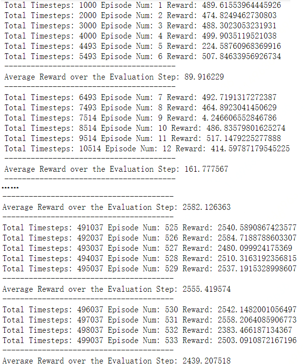
Final render results are shown as follow:
5. Reference
- Addressing Function Approximation Error in Actor-Critic Methods
- OpenAI SpiningUp Documentation-TD3
- Deep Reinforcement Learning 2.0