This post hilights on basic temporal difference learning theory and algorithms that contribute much to more advanced topics like Deep Q Learning (DQN), doublel DQN, dueling DQN and series of Actor-critic methods. Starting from its formulation, and how it is applied in practice.
The post assume that you have basic knowledge of reinforcement learning and Monte Carlo methods for solving RL problem.
1. Temporal Difference Learning Overview
TD learning is a combination of Monte Carlo ideas and dynamic programming (DP) ideas. Like Monte Carlo methods, TD methods can learn directly from raw experience without a model of the environment’s dynamics. Like DP, TD methods update estimates based in part on other learned estimates, without waiting for a final outcome (they bootstrap).
2. Foundmental Topics
As with most basic reforcement learning problem solving technique, we start by interpretating how to make prediction and control based on the prediction.
2.1 TD Prediction
(Reference Rich Sutton) Both TD and Monte Carlo methods use experience to solve the prediction problem. Given some experience following a policy  , both methods update their estimate
  of
of  for the non-terminal states
  occurring in that experience. Monte Carlo methods wait until the return following the visit is known, then use that return as a target for
  . A simple every-visit Monte Carlo method suitable for nonstationary environments is
![\[V\left( {{S_t}} \right) \leftarrow V\left( {{S_t}} \right) + \alpha \left[ {{G_t} - V\left( {{S_t}} \right)} \right]\]](http://www.liaoyong.net/wp-content/ql-cache/quicklatex.com-50dd67760f76b2dad1cce0e184d45239_l3.png "Rendered by QuickLaTeX.com")
where  is the actual return following time
  , and
, and  is a constant step-size parameter, also called constant- MC. Monte Carlo methods must wait until the end of the episode to determine the increment to (only then is known), TD methods need to wait only until the next time step. At time
  they immediately form a target and make a useful update using the observed reward
  and the estimate
  . The simplest TD method makes the update
![\[V\left( {{S_t}} \right) \leftarrow V\left( {{S_t}} \right) + \alpha \left[ {{R_{t + 1}} + \gamma V\left( {{S_{t + 1}}} \right) - V\left( {{S_t}} \right)} \right]\]](http://www.liaoyong.net/wp-content/ql-cache/quicklatex.com-723a37818b04494966bf474dd863d951_l3.png "Rendered by QuickLaTeX.com")
Thus, the target for Monte Carlo update is whereas the target for the TD updates is  .
.
Using TD Learning to evaluate a policy  is as shown in the below box.
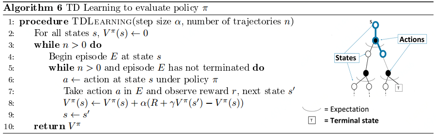 TD Prediction Algorithm:
(1) Initialize  to 0 or some arbitrary values
(2) Begin the episode and for every step in the episode, perform an action  in the state
  and receive a reward
  and move to the next state
(3) Update the value of the previous state using the TD update rule
(4) repeat steps (2) and (3) until reach the terminal state
Attention: In SARSA and Q-learning, we learn  rather than
  .
.
MC method uses the expected value of gains from different episodes to predict the state value function, while TD method use the current next state value and its corresponding reward to update the last state value function.
The above TD methods, or TD(0) bases its update in part on an existing estimate, we say that it is a bootstrapping method. It can learn based on incomplete sequence and update based on the bootstrapping method.
![\[\begin{array}{l} {v_{\rm{\pi }}}\left( s \right) \buildrel\textstyle.\over= {\mathbb{E}_{\rm{\pi }}}\left[ {{G_t}\left| {{S_t} = s} \right.} \right]\\ \;\;\;\;\;\;\;\;{\kern 1pt} = {\mathbb{E}_{\rm{\pi }}}\left[ {\underline {{R_{t + 1}} + \gamma {G_{t + 1}}} \left| {{S_t} = s} \right.} \right]{\kern 1pt} {\kern 1pt} {\kern 1pt} {\kern 1pt} {\kern 1pt} {\kern 1pt} {\kern 1pt} {\kern 1pt} {\kern 1pt} {\kern 1pt} {\kern 1pt} {\kern 1pt} {\kern 1pt} {\kern 1pt} \left( {MC{\kern 1pt} {\kern 1pt} {\kern 1pt} {\rm{Target}}} \right)\\ \;\;\;\;\;\;\;\;{\kern 1pt} = {\mathbb{E}_{\rm{\pi }}}\left[ {\underline {{R_{t + 1}} + \gamma {v_{\rm{\pi }}}\left( {{S_{t + 1}}} \right)} \left| {{S_t} = s} \right.} \right]\;\;\;\;\left( {DP{\kern 1pt} {\kern 1pt} {\rm{Target}}} \right)\\ V\left( {{S_t}} \right) \leftarrow V\left( {{S_t}} \right) + \alpha \left[ {\underline {{R_{t + 1}} + \gamma V\left( {{S_{t + 1}}} \right)} - V\left( {{S_t}} \right)} \right]{\kern 1pt} {\kern 1pt} {\kern 1pt} {\kern 1pt} {\kern 1pt} {\kern 1pt} {\kern 1pt} {\kern 1pt} {\kern 1pt} {\kern 1pt} {\kern 1pt} {\kern 1pt} {\kern 1pt} {\kern 1pt} {\kern 1pt} \left( {TD{\kern 1pt} {\kern 1pt} {\kern 1pt} {\rm{Target}}} \right) \end{array}\]](http://www.liaoyong.net/wp-content/ql-cache/quicklatex.com-3a4cbe14ccdeed38120c579535271219_l3.png "Rendered by QuickLaTeX.com")
The Monte Carlo target is an estimate because the expected value is not known; a sample return is used in place of the real expected return.
The DP target is an estimate not because of the expected values, which are assumed to be completely provided by a model of the environment, but because  is not known and the current estimate,
  , is used instead. The TD target is an estimate for both reasons: it samples the expected values and it uses the current estimate instead of the true
  . Thus, TD methods combine the sampling of Monte Carlo with the bootstrapping of DP.
In TD(0) backup diagram, the value estimate for the state node at the top of the backup diagram is updated on the basis of the one sample transition from it to the immediately following state, as follow:
![]() Sample one transition starting at
Sample one transition starting at  , then we estimate the value of the next state via our current estimate of the next state to construct a full Bellman backup estimate.
The estimation for  follows the same way as above, see details in on-policy SARSA or off-policy Q-learning.
![\[\begin{array}{l} Q\left( {{S_t},{A_t}} \right) \leftarrow Q\left( {{S_t},{A_t}} \right) + \alpha \left[ {{R_{t + 1}} + \gamma Q\left( {{S_{t + 1}},{A_{t + 1}}} \right) - Q\left( {{S_t},{A_t}} \right)} \right]\\ Q\left( {{S_t},{A_t}} \right) \leftarrow Q\left( {{S_t},{A_t}} \right) + \alpha \left[ {{R_{t + 1}} + \gamma \mathop {\max }\limits_a Q\left( {{S_{t + 1}},a} \right) - Q\left( {{S_t},{A_t}} \right)} \right] \end{array}\]](http://www.liaoyong.net/wp-content/ql-cache/quicklatex.com-16b44d98138da094dbbcea8715bcebf0_l3.png "Rendered by QuickLaTeX.com")
TD Error:
The difference between the estimated value of  and the better estimate , as follow:
![\[{\delta _t} \buildrel\textstyle.\over= {R_{t + 1}} + \gamma V\left( {{S_{t + 1}}} \right) - V\left( {{S_t}} \right)\]](http://www.liaoyong.net/wp-content/ql-cache/quicklatex.com-c79fe7a676e76f83b2dd4cf85ca7d0bc_l3.png "Rendered by QuickLaTeX.com")
TD error depends on the next state and next reward, it is not actually available until one time step later. That is,  is the error in , available at time .
Explain by example (TODO):
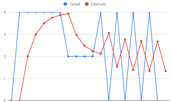
 value in different states can be calculated as follow:
![\[\begin{array}{l} \begin{array}{*{20}{l}} {{R_1} = {q_1} = 0}\\ {{R_2} = 4,{\rm{ }}{q_2} = 0 + 0.5 \times \left( {4 - 0} \right) = 2}\\ {{q_3} = {q_2} + 0.5 \times \left( {{R_2} - {q_2}} \right) = 2 + 0.5 \times \left( {4 - 2} \right) = 3}\\ {{q_4} = {q_3} + 0.5 \times \left( {{R_3} - {q_3}} \right) = 3 + 0.5 \times \left( {4 - 3} \right) = 3.5}\\ { \ldots \ldots }\\ {{q_{15}}{\rm{ }} = {\rm{ }}{q_{14}} + 0.5 \times \left( {{R_{14}} - {q_{14}}} \right) = 1.5 + 0.5 \times \left( {4 - 1.5} \right) = 2.75} \end{array}\\ {q_{16}} = {q_{15}} + 0.5 \times \left( {{R_{15}} - {q_{15}}} \right) = 2.75 + 0.5 \times \left( {0 - 2.75} \right) = 1.35 \end{array}\]](http://www.liaoyong.net/wp-content/ql-cache/quicklatex.com-1dec134821d20ad95a1508f9965075d1_l3.png "Rendered by QuickLaTeX.com")
Advantages of TD methods:
First, compared with DP, they do not require a model of the environment, of its reward and next-state probability distributions; second, compared with MC, they are naturally implemented in an online, fully incremental fashion and wait until the next time-step, which are important in applications of long episodes; Third, TD methods are much less susceptible to problems of ignoring or discounting episodes on which experimental actions are taken, which can greatly slow learning, as in MC Methods.
Tips:
Both TD and Monte Carlo methods converge asymptotically to the correct predictions, however, it is still an open question which method converges faster. In practice, however, TD methods have usually been found to converge faster than constant-α MC methods on stochastic tasks.
2.2 Exploration and Optimality
TD Prediction is used to evaluate state value function, while TD Control is used to improve and optimize the value function, as with Monte Carlo methods, it also need to trade off exploration and exploitation, which results in two kinds of methods, namely, on-policy and off-policy.
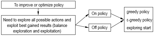 The value of a particular state can be predicted, however, to find best policy or control, some exploration should be made.
Explore with  -greedy method
Balance exploration of suboptimal actions with exploitation of the optimal, or greedy, action. One naive strategy is to take a random action with small probability and take the greedy action the rest of the time. This type of exploration strategy is called an -greedy policy. Mathematically, an -greedy policy with respect to the state-action value  takes the following form:
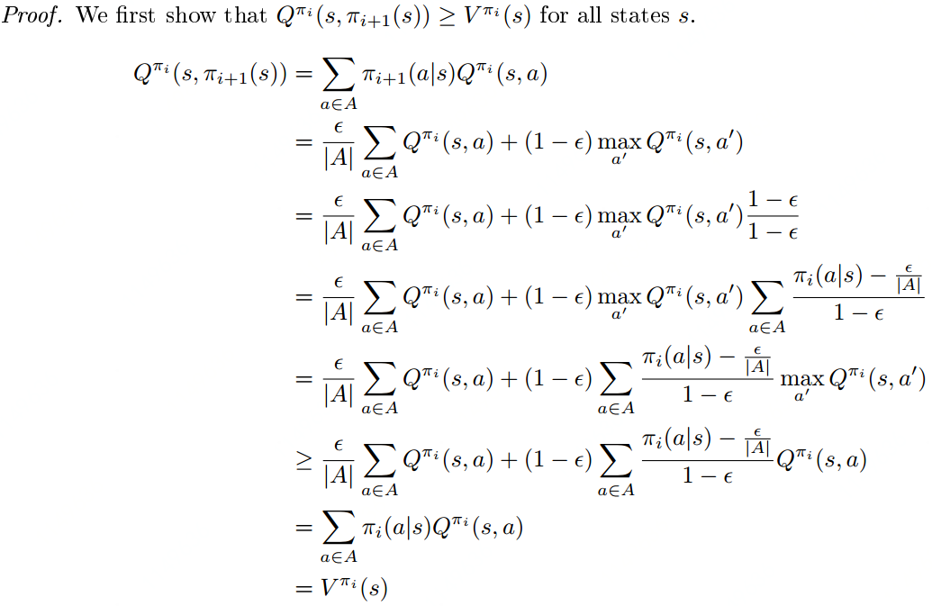
![]() Monotonic -greedy Policy Improvement
Monotonic -greedy Policy Improvement
Let  be an -greedy policy. Then the -greedy policy with respect to
  , denoted
  , is a monotonic improvement on policy . In other words,
  . (Drawn from standford cs234 lecture note).
 Greedy in the limit of exploration
The ε-greedy strategies above is a naive way to balance exploration of new actions with exploitation of current knowledge; however, we can refine this balance by introducing a new class of exploration strategies that allow us to make convergence guarantees about our algorithms. This class of strategies is called Greedy in the Limit of Infinite Exploration (GLIE).
3. On-policy SARSA
SARSA learns an action-value function rather than a state-value function. Learn the values of for all state–action pairs and Sarsa control is an example of GPI with TD learning.
For an on-policy method we must estimate for the current behavior policy and for all states and actions  . This can be done using essentially the same TD method described above for learning
  . Recall that an episode consists of an alternating sequence of states and state–action pairs:
![]() In the previous section we present the transitions from state to state and learned the values of states. Here we consider transitions from state–action pair to state–action pair, and learn the values of state–action pairs, which contributes to policy control. The theorems assuring the convergence of state values under TD(0) also apply to the corresponding algorithm for action values:
In the previous section we present the transitions from state to state and learned the values of states. Here we consider transitions from state–action pair to state–action pair, and learn the values of state–action pairs, which contributes to policy control. The theorems assuring the convergence of state values under TD(0) also apply to the corresponding algorithm for action values:
![\[Q\left( {{S_t},{A_t}} \right) \leftarrow Q\left( {{S_t},{A_t}} \right) + \alpha \left[ {{R_{t + 1}} + \gamma Q\left( {{S_{t + 1}},{A_{t + 1}}} \right) - Q\left( {{S_t},{A_t}} \right)} \right]\]](http://www.liaoyong.net/wp-content/ql-cache/quicklatex.com-e93d6402b2e8456c6a8384632f3ac04f_l3.png "Rendered by QuickLaTeX.com")
This update is done after every transition from a nonterminal state . If  is terminal, then
  is defined as zero. This rule uses every element of the quintuple of events,
 , that make up a transition from one state–action pair to the next.
![]() SARSA gets its name from the parts of the trajectory used in the update equation. To update the Q-value at state-action pair
SARSA gets its name from the parts of the trajectory used in the update equation. To update the Q-value at state-action pair  , we need the reward, next state and next action, thereby using the values
  . SARSA is an on-policy method because the actions and
  used in the update equation are both derived from the policy that is being followed at the time of the update.
As in all on-policy methods, we continually estimate  for the behavior policy , and at the same time change toward greediness with respect to . The general form of the SARSA control algorithm is presented as follow:
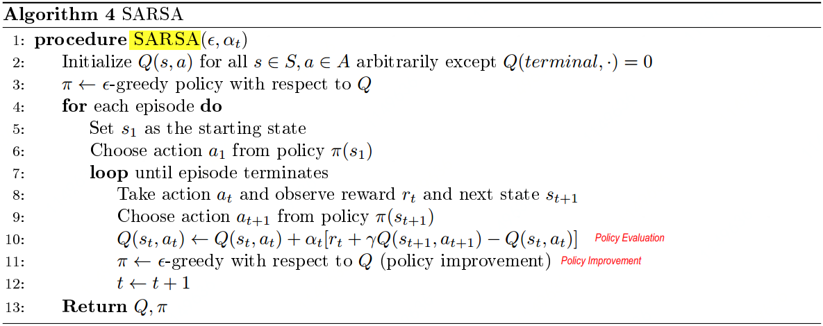 Algorithm description:
(1) initialize the  values to some arbitrary values.
(2) select an action by the epsilon-greedy policy( ) and move from one state to another
(3) update the Q value previous state by following the update rule  , where
  is the action selected y an epsilon-greedy policy(
 ).
).
(4) Repeat (2) and (3) until convergence.
The convergence of SARSA
SARSA converges with probability 1 to an optimal policy and action-value function as long as all state–action pairs are visited an infinite number of times and the policy converges in the limit to the greedy policy.
SARSA for finite-state and finite-action MDP’s converges to the optimal action-value, i.e.  , if the following two conditions hold:
1. The sequence of policies from is GLIE
2. The step-sizes αt satisfy the Robbins-Munro sequence such that
![\[\begin{array}{l} \sum\limits_{t = 1}^\infty {{\alpha _t} = \infty } \\ \sum\limits_{t = 1}^\infty {\alpha _t^2 < \infty } \end{array}\]](http://www.liaoyong.net/wp-content/ql-cache/quicklatex.com-9441ad1387da4aa6bca7f2484e21171a_l3.png "Rendered by QuickLaTeX.com")
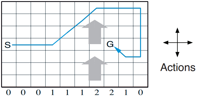
Cases1:Windy Gridworld
Description: refer to Rich Sutton book.
Code implementation:
|
1 2 3 4 5 6 7 8 9 10 11 12 13 14 15 16 17 18 19 20 21 22 23 24 25 26 27 28 29 30 31 32 33 34 35 36 37 38 39 40 41 42 43 44 45 46 47 48 49 50 51 52 53 54 55 56 57 58 59 60 61 62 63 64 65 66 67 68 69 70 71 72 73 74 75 76 77 78 79 80 81 82 83 84 85 86 87 88 89 90 |
import gym import numpy as np from windy_gridworld import WindyGridworldEnv from collections import defaultdict import itertools import sys env = WindyGridworldEnv() state = env.reset() def make_epsilon_greedy_policy(Q, epsilon, nA): """ Creates an epsilon-greedy policy based on a given Q-function and epsilon. Args: Q: A dictionary that maps from state -> action-values. Each value is a numpy array of length nA (see below) epsilon: The probability to select a random action . float between 0 and 1. nA: Number of actions in the environment. Returns: A function that takes the observation as an argument and returns the probabilities for each action in the form of a numpy array of length nA. """ def policy_fn(obseration): A = np.ones(nA, dtype=float) * epsilon / nA best_action = np.argmax(Q[obseration]) A[best_action] += (1.0 - epsilon) return A return policy_fn def sarsa(env, num_episodes, discount_factor=1.0, alpha=0.5, epsilon=0.1): """ SARSA algorithm: On-policy TD control. Finds the optimal epsilon-greedy policy. Args: env: OpenAI environment. num_episodes: Number of episodes to run for. discount_factor: Gamma discount factor. alpha: TD learning rate. epsilon: Chance the sample a random action. Float betwen 0 and 1. Returns: A tuple (Q, stats). Q is the optimal action-value function, a dictionary mapping state -> action values. stats is an EpisodeStats object with two numpy arrays for episode_lengths and episode_rewards. """ # The final action-value function. # A nested dictionary that maps state -> (action -> action-value). Q = defaultdict(lambda: np.zeros(env.action_space.n)) # # Keeps track of useful statistics rewards_set = [] # The policy we're following policy = make_epsilon_greedy_policy(Q, epsilon, env.action_space.n) for i_episode in range(num_episodes): # Print out which episode we're on, useful for debugging. if (i_episode + 1) % 100 == 0: print("\rEpisode {}/{}.".format(i_episode + 1, num_episodes), end="") sys.stdout.flush() episode_reward = 0 # Reset the environment and pick the first action state = env.reset() action_probs = policy(state) action = np.random.choice(np.arange(len(action_probs)), p=action_probs) # One step in the environment for t in itertools.count(): # Take a step next_state, reward, done, _ = env.step(action) # Pick the next action next_action_probs = policy(next_state) next_action = np.random.choice(np.arange(len(next_action_probs)), p=next_action_probs) # Update statistics episode_reward += reward # TD Update td_target = reward + discount_factor * Q[next_state][next_action] td_delta = td_target - Q[state][action] Q[state][action] += alpha * td_delta if done: rewards_set.append(episode_reward) break state = next_state action = next_action return Q, rewards_set Q, rewards_set = sarsa(env, 200) print(rewards_set) |
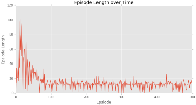
Episode length over time and episode reward over time can be shown as follow:


Case2: Taxi problem code implementation:
|
1 2 3 4 5 6 7 8 9 10 11 12 13 14 15 16 17 18 19 20 21 22 23 24 25 26 27 28 29 30 31 32 33 34 35 36 |
import gym import random env = gym.make('Taxi-v2') alpha = 0.85 gamma = 0.90 epsilon = 0.8 Q = {} #初始化Q值表,用于存储state-action值 for s in range(env.observation_space.n): for a in range(env.action_space.n): Q[(s,a)] = 0.0 def epsilon_greedy(state, epsileon): if random.uniform(0, 1) < epsilon: return env.action_space.sample() else: return max(list(range(env.action_space.n)), key = lambda x:Q[(state, x)]) for i in range(4000): r = 0 #用于存储每个episode的累积奖赏值(comulative reward) state = env.reset() action = epsilon_greedy(state, epsilon) #初始动作选择 while True: next_state, reward, done, _ = env.step(action) #执行动作,进入下一状态 next_action = epsilon_greedy(next_state, epsilon) #选择另一动作值 Q[(state, action)] += alpha * (reward + gamma * Q[(next_state, next_action)] - Q[(state, action)]) #更新上一状态Q值 action = next_action state = next_state r += reward if done: break env.close() |
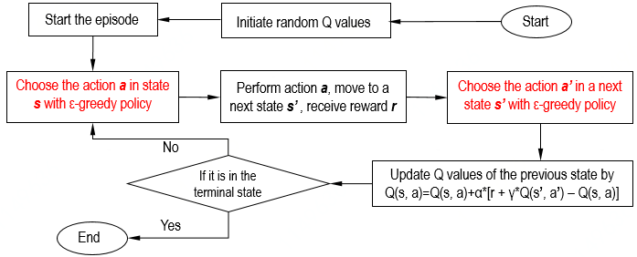
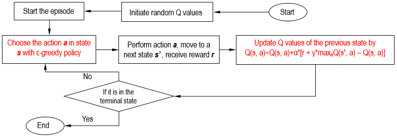
Summary
The flowchart of SARSA is shown as follow:
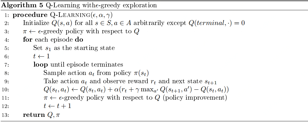
4. Off-policy Q-learning
Q-learning is defined by:
![\[Q\left( {{S_t},{A_t}} \right) \leftarrow Q\left( {{S_t},{A_t}} \right) + \alpha \left[ {{R_{t + 1}} + \gamma \mathop {\max }\limits_a Q\left( {{S_{t + 1}},a} \right) - Q\left( {{S_t},{A_t}} \right)} \right]\]](http://www.liaoyong.net/wp-content/ql-cache/quicklatex.com-ef1b60ac0a3584e69580f7b7b1b490ec_l3.png "Rendered by QuickLaTeX.com")
The learned action-value function, , directly approximates  , the optimal action-value function, independent of the policy being followed. This dramatically simplifies the analysis of the algorithm and enabled early convergence proofs.
Take a maximum over the actions at the next state, this action is not necessarily the same as the one we would derive from the current policy. Q learning algorithm is show in the following box:
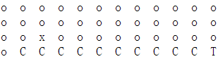
 Case study1: Cliff Walking.
State: grid position of the agent;
Action: movement left, right, up, down;
Reward: -1 on all transition step except those into “The Cliff” region which results in reward of -100 and reset episode.
Refer to Rich Sutton’s book for more detailed description.

Code for the problem using Q-learning is as follow:
|
1 2 3 4 5 6 7 8 9 10 11 12 13 14 15 16 17 18 19 20 21 22 23 24 25 26 27 28 29 30 31 32 33 34 35 36 37 38 39 40 41 42 43 44 45 46 47 48 49 50 51 52 53 54 55 56 57 58 59 60 61 62 63 64 65 66 67 68 69 70 71 72 73 74 75 76 77 78 79 80 81 82 83 84 85 86 |
import numpy as np import gym from collections import defaultdict from cliff_walking import CliffWalkingEnv import itertools env = CliffWalkingEnv() state = env.reset() print(state) def make_epsilon_greedy_policy(Q, epsilon, nA): """ Creates an epsilon-greedy policy based on a given Q-function and epsilon. Args: Q: A dictionary that maps from state -> action-values. Each value is a numpy array of length nA (see below) epsilon: The probability to select a random action. Float between 0 and 1. nA: Number of actions in the environment. Returns: A function that takes the observation as an argument and returns the probabilities for each action in the form of a numpy array of length nA. """ def policy_fn(observation): A = np.ones(nA, dtype=float) * epsilon / nA best_action = np.argmax(Q[observation]) A[best_action] += (1.0 - epsilon) return A return policy_fn def q_learning(env, num_episodes, discount_factor=1.0, alpha=0.5, epsilon=0.1): """ Q-Learning algorithm: Off-policy TD control. Finds the optimal greedy policy while following an epsilon-greedy policy Args: env: OpenAI environment. num_episodes: Number of episodes to run for. discount_factor: Gamma discount factor. alpha: TD learning rate. epsilon: Chance to sample a random action. Float between 0 and 1. Returns: A tuple (Q, episode_lengths). Q is the optimal action-value function, a dictionary mapping state -> action values. stats is an EpisodeStats object with two numpy arrays for episode_lengths and episode_rewards. """ # The final action-value function. # A nested dictionary that maps state -> (action -> action-value) Q = defaultdict(lambda: np.zeros(env.action_space.n)) # The policy we're following rewards_set = [] # The policy we're following policy = make_epsilon_greedy_policy(Q, epsilon, env.action_space.n) for i_episode in range(num_episodes): # Print out which episode we're on, useful for debugging. if (i_episode + 1) % 100 == 0: print("\rEpisode {}/{}.".format(i_episode + 1, num_episodes), end="") sys.stdout.flush() # Reset the environment and pick the first action state = env.reset() episode_reward = 0 # One step in the environment for t in itertools.count(): # Take a step action_probs = policy(state) action = np.random.choice(np.arange(len(action_probs)), p=action_probs) next_state, reward, done, _ = env.step(action) # TD Update td_target = reward + discount_factor * np.max(Q[next_state]) td_delta = td_target - Q[state][action] Q[state][action] += alpha * td_delta episode_reward += reward if done: rewards_set.append(episode_reward) break state = next_state return Q, rewards_set Q, rewards_set = q_learning(env, 600) print(rewards_set) |
Results of the above code implementation are shown as follow:

A speical point here to highlight is that aobve code is based on gym environment, however, we can still build the environment by ourself, as bellow:
(C2M2)
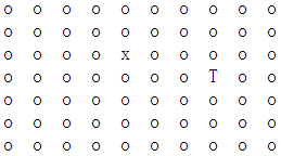
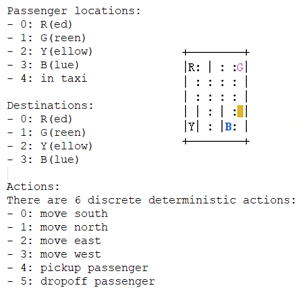
Case Study 2: Taxi Problem
Totaly 500 states,25 taxi positions, 5 possible locations of the passenger (including the case when the passenger is in the taxi), and 4 destination locations.
 Code implementaion:
|
1 2 3 4 5 6 7 8 9 10 11 12 13 14 15 16 17 18 19 20 21 22 23 24 25 26 27 28 29 30 31 32 33 34 35 36 37 38 39 40 |
import random import gym env = gym.make('Taxi-v2') alpha = 0.4 gamma = 0.999 epsilon = 0.017 q = {} for s in range(env.observation_space.n): for a in range(env.action_space.n): q[(s, a)] = 0 def update_q_table(prev_state, action, reward, next_state, alpha, gamma): qa = max([q[next_state, a] for a in range(env.action_space.n)]) #取action最大值 q[(prev_state, action)] += alpha * (reward + gamma * qa - q[(prev_state, action)]) def epsilon_greedy_policy(state, epsilon): if random.uniform(0, 1) < epsilon: return env.action_space.sample() else: return max(list(range(env.action_space.n)), key = lambda x: q[(state, x)]) for i in range(8000): r = 0 prev_state = env.reset() #状态索引值,如88 while True: env.render() action = epsilon_greedy_policy(prev_state, epsilon) next_state, reward, done, _ = env.step(action) update_q_table(prev_state, action, reward, next_state, alpha, gamma) prev_state = next_state r += reward if done: break print("total rewward: ", r) env.close() |
Compare Q-learning with SARSA
In Q-learning, we take action using an epsilon-greedy policy and simply pick up the maximum action to update the Q value, while in SARSA, we take action using the epsilon-greedy policy and also pick up the action using the epsilon-greedy policy to update the Q value.
Q-learning is off-policy because it updates its Q-values using the Q-values of the next state and the greedy action . It estimates the return (total discounted future reward) for state-action pairs assuming a greedy policy were followed depite that fact that it’s not follwing a greedy policy. SARSA is on-policy since it updates its Q-values using the Q-value of the next state and the current policy’s action  . It estimates the return for state-action pairs assuming the current policy continues to be followed. The distinction disappears if the current policy is a greedy policy.
Summary
Algorithm flow is as follow:
5. Off-policy Expected SARSA
Rather than sampling from to pick an action , we should just calculate the expected value of  . This way, the estimate of how good is won’t fluctuate around, like it would when sampling an action from a distribution, but rather remain steady around the “average” outcome for the state.
The corresponding algorithm pseudocode is as follow:
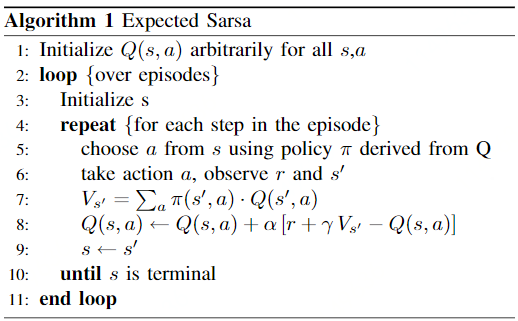 The update rule in expected SARSA is
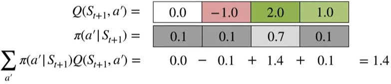
![\[\begin{array}{l} Q\left( {{S_t},{A_t}} \right) \leftarrow Q\left( {{S_t},{A_t}} \right) + \alpha \left[ {{R_{t + 1}} + \gamma {E_{\rm{\pi }}}\left[ {Q\left( {{S_{t + 1}},{A_{t + 1}}} \right)\left| {{S_{t + 1}}} \right.} \right] - Q\left( {{S_t},{A_t}} \right)} \right]\\ {\kern 1pt} {\kern 1pt} {\kern 1pt} {\kern 1pt} {\kern 1pt} {\kern 1pt} {\kern 1pt} {\kern 1pt} {\kern 1pt} {\kern 1pt} {\kern 1pt} {\kern 1pt} {\kern 1pt} {\kern 1pt} {\kern 1pt} {\kern 1pt} {\kern 1pt} {\kern 1pt} {\kern 1pt} {\kern 1pt} {\kern 1pt} {\kern 1pt} {\kern 1pt} {\kern 1pt} {\kern 1pt} {\kern 1pt} {\kern 1pt} {\kern 1pt} {\kern 1pt} {\kern 1pt} {\kern 1pt} {\kern 1pt} {\kern 1pt} {\kern 1pt} {\kern 1pt} {\kern 1pt} {\kern 1pt} {\kern 1pt} {\kern 1pt} {\kern 1pt} {\kern 1pt} {\kern 1pt} {\kern 1pt} {\kern 1pt} {\kern 1pt} {\kern 1pt} \leftarrow Q\left( {{S_t},{A_t}} \right) + \alpha \left[ {{R_{t + 1}} + \gamma \sum\limits_{a'} {{\rm{\pi }}\left( {a'\left| {{S_{t + 1}}} \right.} \right)Q\left( {{S_{t + 1}},a'} \right)} - Q\left( {{S_t},{A_t}} \right)} \right] \end{array}\]](http://www.liaoyong.net/wp-content/ql-cache/quicklatex.com-c7c8d723e17967dd53f979c389afa14b_l3.png "Rendered by QuickLaTeX.com")
A calculation illustration:
 Code implementation (C2M3):
6. Summary
Till now, we have goen through the temporal difference learning approches and seen how the Bellman equation is used to form these on-policy or off-policy algorithm, understanding idea of these basic algorithms is important to decompose more advanced methods later.