Background
The loss weights are uniform or manually tuned.
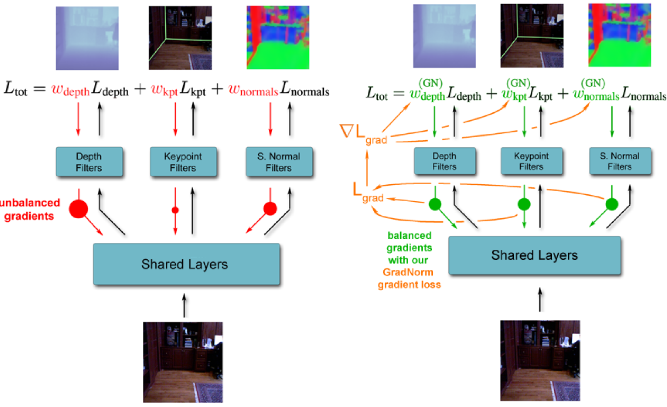
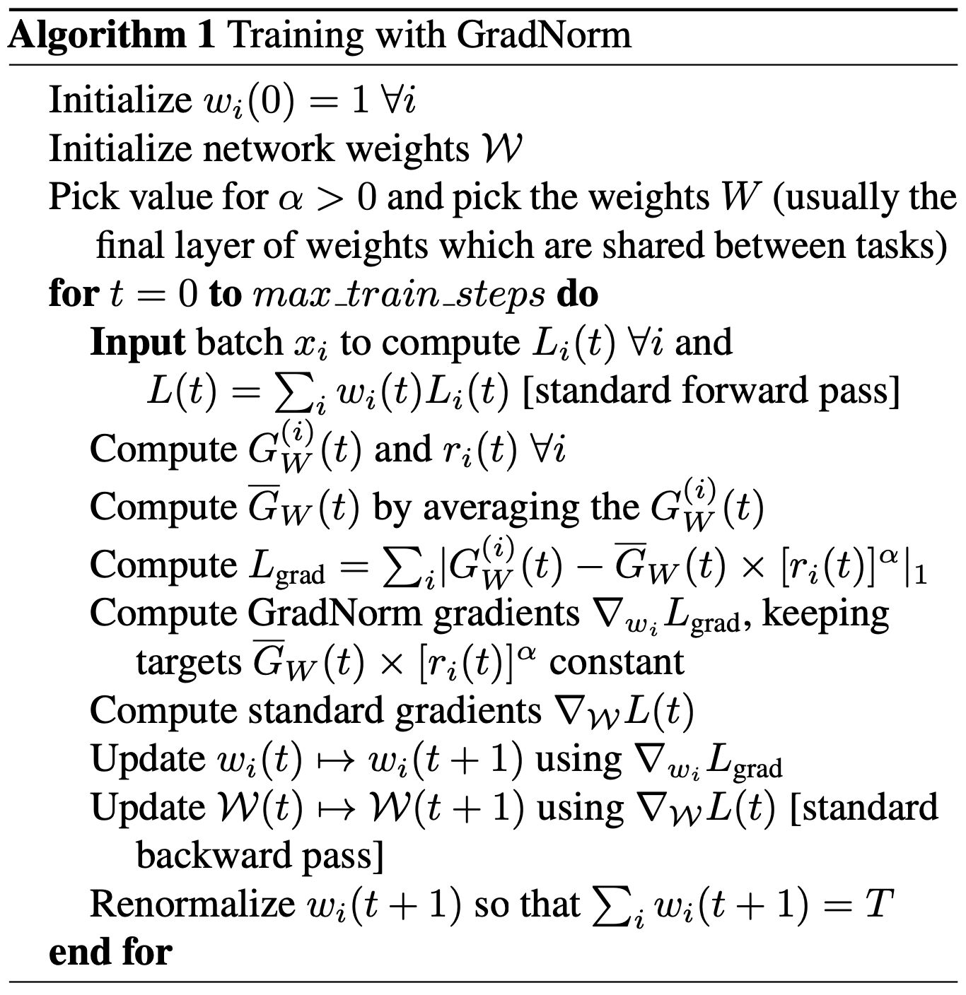
GradNorm
GradNorm: Gradient Normalization for Adaptive Loss Balancing in Deep Multitask Networks
Task imbalances impede proper training because they manifest as imbalances between backpropagated gradients.
Assume the linear form of the loss function.
The multi-task loss formulation: 
Notations:
 : The subset of the full network weights
  , the network weight parameters that updated by GradNorm and is generally chosen as the last shared layer of weights.
 : the
: the  norm of the gradient of the weighted single-task loss
  with respect to the chosen weights .
![\bar{G}_{W}(t)=E_{\mathrm{task}}\left[G_{W}^{(i)}(t)\right]](http://www.liaoyong.net/wp-content/ql-cache/quicklatex.com-dbfc2f66231fb0cbbb725fe32ecea260_l3.png "Rendered by QuickLaTeX.com") : the average gradient norm across all tasks at training time {t}.
: the average gradient norm across all tasks at training time {t}.
 : the loss ratio for task
  at time
  ,
,  is a measure of the inverse training rate of task (i.e. lower values of correspond to a faster training rate for task ).
![r_{i}(t)=\tilde{L}_{i}(t) / E_{\text {task }}\left[\tilde{L}_{i}(t)\right]](http://www.liaoyong.net/wp-content/ql-cache/quicklatex.com-cf8f77ec6cb38b35876357ff62cfdf71_l3.png "Rendered by QuickLaTeX.com") : the relative reverse training rate for task .
: the relative reverse training rate for task .
The higher the value of  , the higher the gradient magnitudes should be for task in order to encourage the task to train more quickly. So the desired or target gradient norm for each task is :
![\[ G_{W}^{(i)}(t) \mapsto \bar{G}_{W}(t) \times\left[r_{i}(t)\right]^{\alpha} \]](http://www.liaoyong.net/wp-content/ql-cache/quicklatex.com-a4b6aad50fda6f31b682ab53874769a3_l3.png "Rendered by QuickLaTeX.com")
The loss weight  is updated by minimizing the
  loss
loss  of between the actual and target gradient norms at each time-step for each task, summed over all tasks.
![\[ L_{\mathrm{grad}}\left(t ; w_{i}(t)\right)=\sum_{i}\left|G_{W}^{(i)}(t)-\bar{G}_{W}(t) \times\left[r_{i}(t)\right]^{\alpha}\right|_{1} \]](http://www.liaoyong.net/wp-content/ql-cache/quicklatex.com-1d41c8933b145dc83c9b4d3f3d234487_l3.png "Rendered by QuickLaTeX.com")
is differentiated only with respect to the , the computed gradients  are then applied via standard update rules to update each .
Code implementation
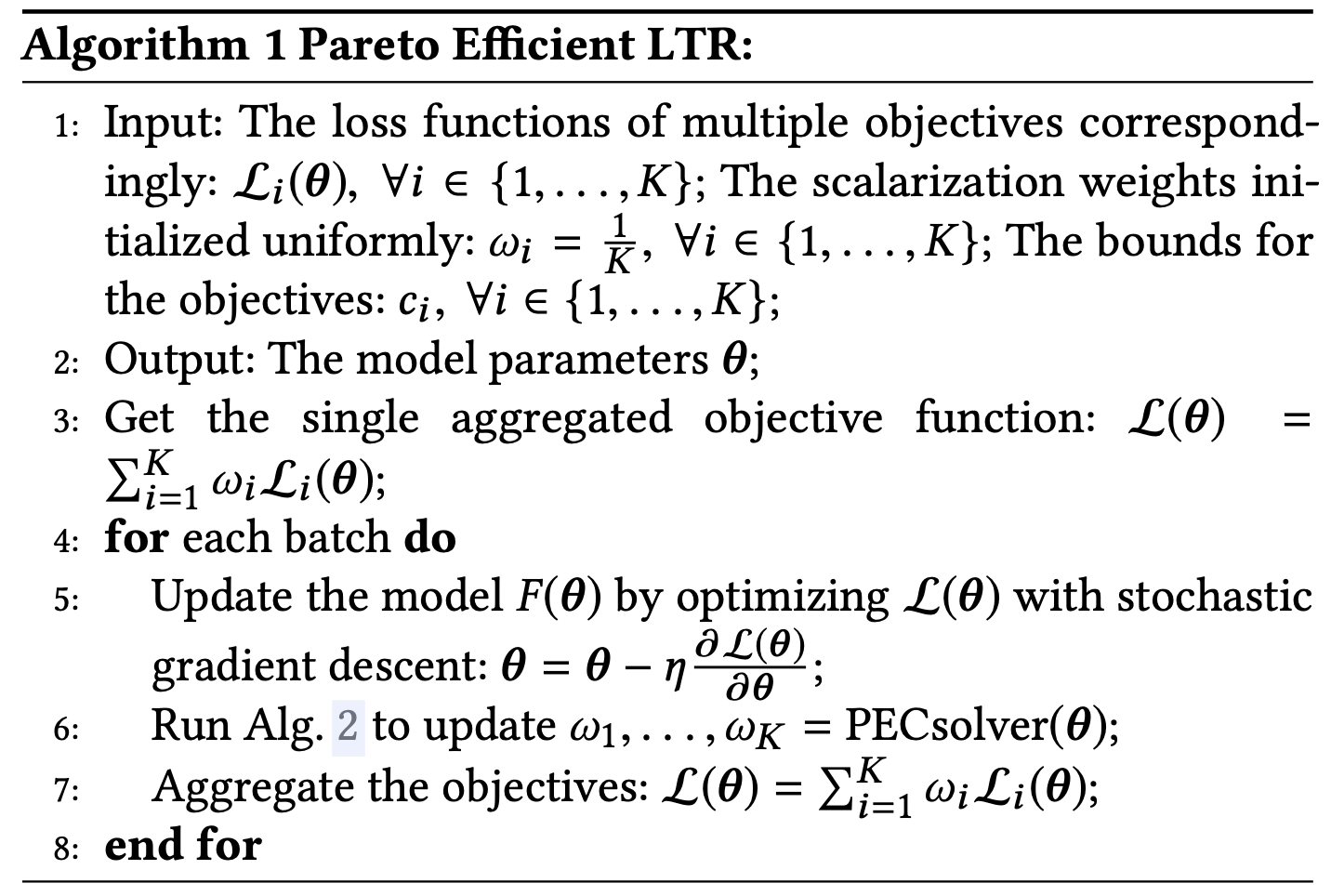
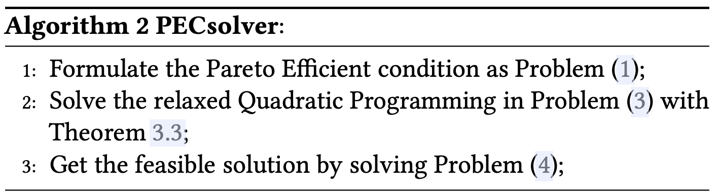
PE-LTR
![\[ \mathcal{L}(\boldsymbol{\theta})=\sum_{i=1}^{K} \omega_{i} \mathcal{L}_{i}(\boldsymbol{\theta}) \]](http://www.liaoyong.net/wp-content/ql-cache/quicklatex.com-80867d48bee27175b378349468eb93d3_l3.png "Rendered by QuickLaTeX.com")
where
![\[ \sum_{i=1}^{K} \omega_{i}=1, \quad \exists \omega_{i} \geq c_{i}, i \in\{1, \ldots, K\} \text { and } \sum_{i=1}^{K} \omega_{i} \nabla_{\boldsymbol{\theta}} \mathcal{L}_{i}(\boldsymbol{\theta})=0 \]](http://www.liaoyong.net/wp-content/ql-cache/quicklatex.com-a8e857c8a65096d6c680ac381cdcdd0c_l3.png "Rendered by QuickLaTeX.com")
![\[ \begin{aligned} &\min \cdot\left\|\sum_{i=1}^{K} \omega_{i} \nabla_{\boldsymbol{\theta}} \mathcal{L}_{i}(\boldsymbol{\theta})\right\|_{2}^{2} \\ &\text { s.t. } \sum_{i=1}^{K} \omega_{i}=1, \omega_{i} \geq c_{i}, \forall i \in\{1, \ldots, K\} \end{aligned} \]](http://www.liaoyong.net/wp-content/ql-cache/quicklatex.com-12f8033ec172baeb3c5a434cfc803c56_l3.png "Rendered by QuickLaTeX.com")
![\[ \begin{aligned} \min \cdot &\left\|\sum_{i=1}^{K}\left(\hat{\omega}_{i}+c_{i}\right) \nabla_{\boldsymbol{\theta}} \mathcal{L}_{i}(\boldsymbol{\theta})\right\|_{2}^{2} \\ \text { s.t. } & \sum_{i=1}^{K} \hat{\omega}_{i}=1-\sum_{i=1}^{K} c_{i}, \hat{\omega}_{i} \geq 0, \forall i \in\{1, \ldots, K\} \end{aligned} \]](http://www.liaoyong.net/wp-content/ql-cache/quicklatex.com-edbba328810819ee9257b5fbc7464bc8_l3.png "Rendered by QuickLaTeX.com")
![]()
![\[ \min \cdot\left\|\tilde{\omega}-\hat{\omega}^{*}\right\|_{2}^{2} \text { s.t. } \sum_{i=1}^{K} \tilde{\omega}_{i}=1, \tilde{\omega}_{i} \geq 0, \forall i \in\{1, \ldots, K\} \]](http://www.liaoyong.net/wp-content/ql-cache/quicklatex.com-b1ab8d6171ddca685eae5b07b956026b_l3.png "Rendered by QuickLaTeX.com")
 Code Implementation
|
1 2 3 4 5 6 7 8 9 10 11 12 13 14 15 16 17 18 19 20 21 22 23 24 25 26 27 28 29 30 31 32 33 34 35 36 37 38 39 40 41 42 43 44 45 46 47 48 49 50 51 52 53 54 55 56 57 58 59 60 61 62 63 64 65 66 67 68 69 70 71 72 73 74 |
import tensorflow as tf import numpy as np from scipy.optimize import minimize from scipy.optimize import nnls seed = 3456 tf.set_random_seed(seed) np.random.seed(seed) x_data = np.float32(np.random.rand(100, 4)) y_data = np.dot(x_data, [[0.100], [0.200], [0.300], [0.400]]) + 0.300 weight_a = tf.placeholder(tf.float32) weight_b = tf.placeholder(tf.float32) b = tf.Variable(tf.zeros([1])) W = tf.Variable(tf.random_uniform([4, 1], -1.0, 1.0)) y = tf.matmul(x_data, W) + b loss_a = tf.reduce_mean(tf.square(y - y_data)) loss_b = tf.reduce_mean(tf.square(W) + tf.square(b)) loss = weight_a * loss_a + weight_b * loss_b optimizer = tf.train.GradientDescentOptimizer(0.1) a_grad = tf.gradients(loss_a, W) b_grad = tf.gradients(loss_b, W) train = optimizer.minimize(loss) init = tf.initialize_all_variables() sess = tf.Session() sess.run(init) def pareto_step(w, c, G): GGT = np.matmul(G, np.transpose(G)) e = np.mat(np.ones(np.shape(w))) m_up = np.hstack((GGT, e)) m_down = np.hstack((np.transpose(e), np.mat(np.zeros((1, 1))))) M = np.vstack((m_up, m_down)) z = np.vstack((-np.matmul(GGT, c), 1 - np.sum(c))) hat_w = np.matmul(np.matmul(np.linalg.inv(np.matmul(np.transpose(M),M)), M), z) hat_w = hat_w[:-1] hat_w = np.reshape(np.array(hat_w), (hat_w.shape[0],)) c = np.reshape(np.array(c), (c.shape[0],)) new_w = ASM(hat_w, c) return new_w def ASM(hat_w, c): A = np.array([[0 if i != j else 1 for i in range(len(c))] for j in range(len(c))]) b = hat_w x0, _ = nnls(A, b) def _fn(x, A, b): return np.linalg.norm(A.dot(x) - b) cons = {'type': 'eq', 'fun': lambda x: np.sum(x) + np.sum(c) - 1} bounds = [[0, None] for _ in range(len(hat_w))] min_out = minimize(_fn, x0, args=(A, b), method='SLSQP', bounds=bounds, constraints=cons) new_w = min_out.x + c return new_w w_a, w_b = 0.5, 0.5 c_a, c_b = 0.2, 0.2 for step in range(0, 10): res = sess.run([a_grad, b_grad, train], feed_dict={weight_a: w_a, weight_b: w_b}) print('-----------------------step {} ---------------------'.format(str(step))) print(res) weights = np.mat([[w_a], [w_b]]) print(weights) paras = np.hstack((res[0][0], res[1][0])) # G: stack gradient wrt W print(paras) paras = np.transpose(paras) w_a, w_b = pareto_step(weights, np.mat([[c_a], [c_b]]), paras) la = sess.run(loss_a) lb = sess.run(loss_b) print("{:0>2d} {:4f} {:4f} {:4f} {:4f} {:4f}".format(step, w_a, w_b, la, lb, la / lb)) |
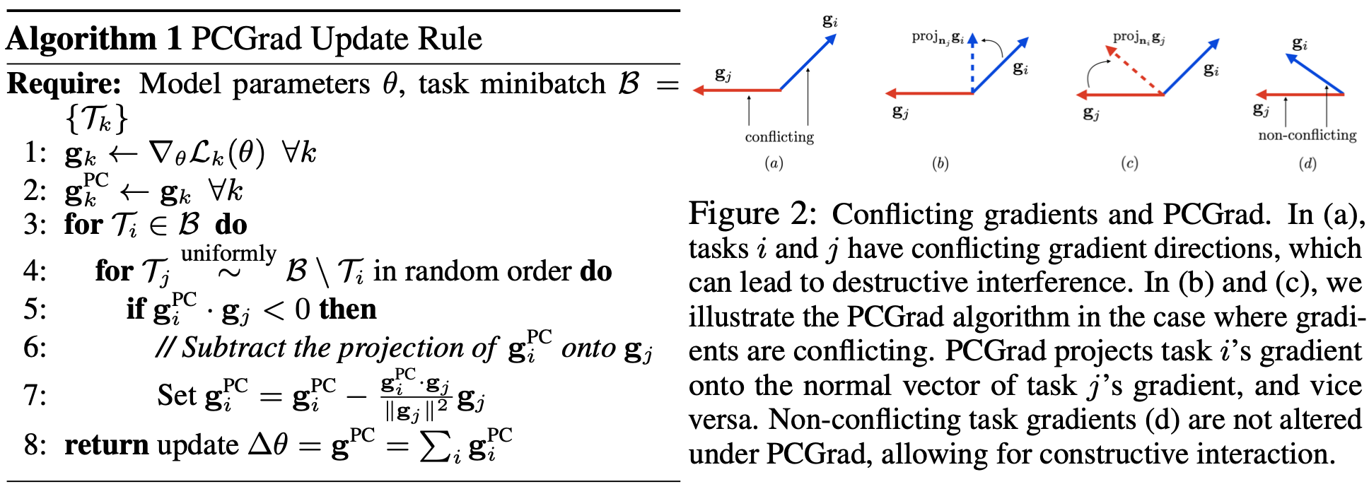
PCGrad
|
1 2 3 4 5 6 7 8 9 10 11 12 13 14 15 16 17 18 19 20 21 22 23 24 25 26 27 28 29 30 31 32 33 34 35 36 37 38 39 40 41 42 43 44 45 46 47 48 49 50 51 52 53 54 55 56 57 58 59 60 61 62 63 64 65 66 67 68 69 70 71 72 73 74 75 76 77 78 79 80 81 82 83 84 85 86 87 88 89 90 91 92 93 94 95 96 97 98 99 |
from __future__ import absolute_import from __future__ import division from __future__ import print_function import numpy as np import random import tensorflow as tf from tensorflow.python.eager import context from tensorflow.python.framework import ops from tensorflow.python.ops import control_flow_ops from tensorflow.python.training import optimizer GATE_OP = 1 class PCGrad(optimizer.Optimizer): '''Tensorflow implementation of PCGrad. Gradient Surgery for Multi-Task Learning: https://arxiv.org/pdf/2001.06782.pdf ''' def __init__(self, optimizer, use_locking=False, name="PCGrad"): """optimizer: the optimizer being wrapped """ super(PCGrad, self).__init__(use_locking, name) self.optimizer = optimizer def compute_gradients(self, loss, var_list=None, gate_gradients=GATE_OP, aggregation_method=None, colocate_gradients_with_ops=False, grad_loss=None): assert type(loss) is list num_tasks = len(loss) loss = tf.stack(loss) tf.random.shuffle(loss) # Compute per-task gradients. grads_task = tf.vectorized_map(lambda x: tf.concat([tf.reshape(grad, [-1,]) for grad in tf.gradients(x, var_list) if grad is not None], axis=0), loss) # Compute gradient projections. def proj_grad(grad_task): for k in range(num_tasks): inner_product = tf.reduce_sum(grad_task*grads_task[k]) proj_direction = inner_product / tf.reduce_sum(grads_task[k]*grads_task[k]) grad_task = grad_task - tf.minimum(proj_direction, 0.) * grads_task[k] return grad_task proj_grads_flatten = tf.vectorized_map(proj_grad, grads_task) # Unpack flattened projected gradients back to their original shapes. proj_grads = [] for j in range(num_tasks): start_idx = 0 for idx, var in enumerate(var_list): grad_shape = var.get_shape() flatten_dim = np.prod([grad_shape.dims[i].value for i in range(len(grad_shape.dims))]) proj_grad = proj_grads_flatten[j][start_idx:start_idx+flatten_dim] proj_grad = tf.reshape(proj_grad, grad_shape) if len(proj_grads) < len(var_list): proj_grads.append(proj_grad) else: proj_grads[idx] += proj_grad start_idx += flatten_dim grads_and_vars = list(zip(proj_grads, var_list)) return grads_and_vars def _create_slots(self, var_list): self.optimizer._create_slots(var_list) def _prepare(self): self.optimizer._prepare() def _apply_dense(self, grad, var): return self.optimizer._apply_dense(grad, var) def _resource_apply_dense(self, grad, var): return self.optimizer._resource_apply_dense(grad, var) def _apply_sparse_shared(self, grad, var, indices, scatter_add): return self.optimizer._apply_sparse_shared(grad, var, indices, scatter_add) def _apply_sparse(self, grad, var): return self.optimizer._apply_sparse(grad, var) def _resource_scatter_add(self, x, i, v): return self.optimizer._resource_scatter_add(x, i, v) def _resource_apply_sparse(self, grad, var, indices): return self.optimizer._resource_apply_sparse(grad, var, indices) def _finish(self, update_ops, name_scope): return self.optimizer._finish(update_ops, name_scope) def _call_if_callable(self, param): """Call the function if param is callable.""" return param() if callable(param) else param |
Uncertainty Weighting
Joint learning the regression and classification tasks with different units and scales.
The optimal weighting loss of each task is dependent on the measurement scale (e.g. meters, centimetres or millimetres) and ultimately the magnitude of the task’s noise.
In the case of multiple model outputs, we often define the likelihood to factorize over the outputs, given some sufficient statistics.
In typical multi-task learning, the total loss is the weighted linear sum of the losses for each task:
![\[ L_{\text {total }}=\sum_{i} w_{i} L_{i} \]](http://www.liaoyong.net/wp-content/ql-cache/quicklatex.com-ec76deab2aae72d70efa515d86b342c8_l3.png "Rendered by QuickLaTeX.com")
For regression task with outputs  , the likelihood is defined as Gaussian with mean given by and an observation noise scalar
  .
.
![\[ p\left(\mathbf{y} \mid \mathbf{f}^{\mathbf{W}}(\mathbf{x})\right)=\mathcal{N}\left(\mathbf{f}^{\mathbf{W}}(\mathbf{x}), \sigma^{2}\right) \]](http://www.liaoyong.net/wp-content/ql-cache/quicklatex.com-f72a4cc85a1a8c948ec5b7e01394a8d5_l3.png "Rendered by QuickLaTeX.com")
For classification task, the model output is passed into the Softmax function to get the probabilty.
![\[ p\left(\mathbf{y} \mid \mathbf{f}^{\mathbf{W}}(\mathbf{x})\right)=\operatorname{Softmax}\left(\mathbf{f}^{\mathbf{W}}(\mathbf{x})\right) \]](http://www.liaoyong.net/wp-content/ql-cache/quicklatex.com-c6a59d46268ec2e6b3d3f69a9bab9aa8_l3.png "Rendered by QuickLaTeX.com")
Generally, the multi-task likelihood is formed by factorizing overing the outputs assuming the to be the sufficient statistics, denoted as bellow:
![\[ p\left(\mathbf{y}_{1}, \ldots, \mathbf{y}_{K} \mid \mathbf{f}^{\mathbf{W}}(\mathbf{x})\right)=p\left(\mathbf{y}_{1} \mid \mathbf{f}^{\mathbf{W}}(\mathbf{x})\right) \ldots p\left(\mathbf{y}_{K} \mid \mathbf{f}^{\mathbf{W}}(\mathbf{x})\right) \]](http://www.liaoyong.net/wp-content/ql-cache/quicklatex.com-fa558e86d7bbb08abfedaf4a594b2a53_l3.png "Rendered by QuickLaTeX.com")
In maximum likelihood inference, we maximize the log likelihood of the model, take the regression task for example:
![\[ \log p\left(\mathbf{y} \mid \mathbf{f}^{\mathbf{W}}(\mathbf{x})\right) \propto-\frac{1}{2 \sigma^{2}}\left\|\mathbf{y}-\mathbf{f}^{\mathbf{w}}(\mathbf{x})\right\|^{2}-\log \sigma \]](http://www.liaoyong.net/wp-content/ql-cache/quicklatex.com-b1788cfe920e55d6013cea5d8197263e_l3.png "Rendered by QuickLaTeX.com")
![\[ \begin{aligned} p\left(\mathbf{y}_{1}, \mathbf{y}_{2} \mid \mathbf{f}^{\mathbf{W}}(\mathbf{x})\right) &=p\left(\mathbf{y}_{1} \mid \mathbf{f}^{\mathbf{W}}(\mathbf{x})\right) \cdot p\left(\mathbf{y}_{2} \mid \mathbf{f}^{\mathbf{W}}(\mathbf{x})\right) \\ &=\mathcal{N}\left(\mathbf{y}_{1} ; \mathbf{f}^{\mathbf{W}}(\mathbf{x}), \sigma_{1}^{2}\right) \cdot \mathcal{N}\left(\mathbf{y}_{2} ; \mathbf{f}^{\mathbf{W}}(\mathbf{x}), \sigma_{2}^{2}\right) \end{aligned} \]](http://www.liaoyong.net/wp-content/ql-cache/quicklatex.com-f64fdc1705ae945f6ce2a4f960fa7eb8_l3.png "Rendered by QuickLaTeX.com")
Minimize objective:
![\[ \begin{aligned} &=-\log p\left(\mathbf{y}_{1}, \mathbf{y}_{2} \mid \mathbf{f}^{\mathbf{W}}(\mathbf{x})\right) \\ &\propto \frac{1}{2 \sigma_{1}^{2}}\left\|\mathbf{y}_{1}-\mathbf{f}^{\mathbf{W}}(\mathbf{x})\right\|^{2}+\frac{1}{2 \sigma_{2}^{2}}\left\|\mathbf{y}_{2}-\mathbf{f}^{\mathbf{W}}(\mathbf{x})\right\|^{2}+\log \sigma_{1} \sigma_{2} \\ &=\frac{1}{2 \sigma_{1}^{2}} \mathcal{L}_{1}(\mathbf{W})+\frac{1}{2 \sigma_{2}^{2}} \mathcal{L}_{2}(\mathbf{W})+\log \sigma_{1} \sigma_{2} \end{aligned} \]](http://www.liaoyong.net/wp-content/ql-cache/quicklatex.com-76c04b6a34e4af1129b61bf4cf8e09ab_l3.png "Rendered by QuickLaTeX.com")
For classification problem,
![\[ p\left(\mathbf{y} \mid \mathbf{f}^{\mathbf{W}}(\mathbf{x}), \sigma\right)=\operatorname{Softmax}\left(\frac{1}{\sigma^{2}} \mathbf{f}^{\mathbf{W}}(\mathbf{x})\right) \]](http://www.liaoyong.net/wp-content/ql-cache/quicklatex.com-b90d2a0c31c5771894c99649d4ec22f9_l3.png "Rendered by QuickLaTeX.com")
![\[ \begin{aligned} \log p\left(\mathbf{y}=c \mid \mathbf{f}^{\mathbf{W}}(\mathbf{x}), \sigma\right) &=\frac{1}{\sigma^{2}} f_{c}^{\mathbf{W}}(\mathbf{x}) \\ &-\log \sum_{c^{\prime}} \exp \left(\frac{1}{\sigma^{2}} f_{c^{\prime}}^{\mathbf{W}}(\mathbf{x})\right) \end{aligned} \]](http://www.liaoyong.net/wp-content/ql-cache/quicklatex.com-040b5c30c6f3f78055cc9e618b92a0e3_l3.png "Rendered by QuickLaTeX.com")
Combination of regression and classification problem:
![\[ \begin{aligned} &=-\log p\left(\mathbf{y}_{1}, \mathbf{y}_{2}=c \mid \mathbf{f}^{\mathbf{W}}(\mathbf{x})\right) \\ &=-\log \mathcal{N}\left(\mathbf{y}_{1} ; \mathbf{f}^{\mathbf{W}}(\mathbf{x}), \sigma_{1}^{2}\right) \cdot \operatorname{Softmax}\left(\mathbf{y}_{2}=c ; \mathbf{f}^{\mathbf{W}}(\mathbf{x}), \sigma_{2}\right) \\ &=\frac{1}{2 \sigma_{1}^{2}}\left\|\mathbf{y}_{1}-\mathbf{f}^{\mathbf{W}}(\mathbf{x})\right\|^{2}+\log \sigma_{1}-\log p\left(\mathbf{y}_{2}=c \mid \mathbf{f}^{\mathbf{W}}(\mathbf{x}), \sigma_{2}\right) \\ &=\frac{1}{2 \sigma_{1}^{2}} \mathcal{L}_{1}(\mathbf{W})+\frac{1}{\sigma_{2}^{2}} \mathcal{L}_{2}(\mathbf{W})+\log \sigma_{1} \\ &\quad+\log \frac{\sum_{c^{\prime}} \exp \left(\frac{1}{\sigma_{2}^{2}} f_{c^{\prime}}^{\mathbf{W}}(\mathbf{x})\right)}{\left(\sum_{c^{\prime}} \exp \left(f_{c^{\prime}}^{\mathbf{W}}(\mathbf{x})\right)\right)^{\frac{1}{\sigma_{2}^{2}}}} \\ &\approx \frac{1}{2 \sigma_{1}^{2}} \mathcal{L}_{1}(\mathbf{W})+\frac{1}{\sigma_{2}^{2}} \mathcal{L}_{2}(\mathbf{W})+\log \sigma_{1}+\log \sigma_{2} \end{aligned} \]](http://www.liaoyong.net/wp-content/ql-cache/quicklatex.com-39ef4969272166aa0eb41ae868effe8f_l3.png "Rendered by QuickLaTeX.com")
Code implementation
|
1 2 3 4 5 6 7 8 9 10 11 12 13 14 15 16 17 18 19 20 21 22 23 24 25 26 27 28 29 30 31 32 33 34 35 36 37 38 39 40 41 42 43 44 45 46 47 48 49 50 51 52 53 54 55 56 57 58 59 60 61 62 63 64 65 66 67 68 |
import tensorflow as tf from utils.utils import accuracy slim = tf.contrib.slim FLAGS = tf.app.flags.FLAGS class MultiLossLayer(): def __init__(self, loss_list): self._loss_list = loss_list self._sigmas_sq = [] for i in range(len(self._loss_list)): self._sigmas_sq.append(slim.variable('Sigma_sq_' + str(i), dtype=tf.float32, shape=[], initializer=tf.initializers.random_uniform(minval=0.2, maxval=1))) def get_loss(self): factor = tf.div(1.0, tf.multiply(2.0, self._sigmas_sq[0])) loss = tf.add(tf.multiply(factor, self._loss_list[0]), tf.log(self._sigmas_sq[0])) for i in range(1, len(self._sigmas_sq)): factor = tf.div(1.0, tf.multiply(2.0, self._sigmas_sq[i])) loss = tf.add(loss, tf.add(tf.multiply(factor, self._loss_list[i]), tf.log(self._sigmas_sq[i]))) return loss def get_loss(logits, ground_truths): multi_loss_class = None loss_list = [] if FLAGS.task1: label_type = ground_truths[0] loss_list.append(loss(logits[0], label_type, type='cross_entropy')) if FLAGS.use_label_inst: xy_gt = tf.slice(ground_truths[1], [0, 0, 0, 0], [-1, FLAGS.output_height, FLAGS.output_width, 2]) # to get x GT and y GT mask = tf.slice(ground_truths[1], [0, 0, 0, 2], [-1, FLAGS.output_height, FLAGS.output_width, 1]) # to get mask from GT mask = tf.concat([mask, mask], 3) # to get mask for x and for y if FLAGS.need_resize: xy_gt = tf.image.resize_images(xy_gt, [FLAGS.output_height, FLAGS.output_width], method=tf.image.ResizeMethod.BILINEAR, align_corners=False) mask = tf.image.resize_images(mask, [FLAGS.output_height, FLAGS.output_width], method=tf.image.ResizeMethod.BILINEAR, align_corners=False) loss_list.append(l1_masked_loss(tf.multiply(logits[1], mask), xy_gt, mask)) if FLAGS.use_label_disp: if FLAGS.need_resize: gt_sized = tf.image.resize_images(ground_truths[2], [FLAGS.output_height, FLAGS.output_width], method=tf.image.ResizeMethod.BILINEAR, align_corners=False) gt_sized = gt_sized[:, :, :, 0] mask = gt_sized[:, :, :, 1] else: gt_sized = tf.expand_dims(ground_truths[2][:, :, :, 0], axis=-1) mask = tf.expand_dims(ground_truths[2][:, :, :, 1], axis=-1) loss_list.append(l1_masked_loss(tf.multiply(logits[2], mask), tf.multiply(gt_sized, mask), mask)) if FLAGS.use_multi_loss: loss_op, multi_loss_class = calc_multi_loss(loss_list) else: loss_op = loss_list[0] for i in range(1, len(loss_list)): loss_op = tf.add(loss_op, loss_list[i]) return loss_op, loss_list, multi_loss_class def calc_multi_loss(loss_list): multi_loss_layer = MultiLossLayer(loss_list) return multi_loss_layer.get_loss(), multi_loss_layer def l1_masked_loss(logits, gt, mask): valus_diff = tf.abs(tf.subtract(logits, gt)) L1_loss = tf.divide(tf.reduce_sum(valus_diff), tf.add(tf.reduce_sum(mask[:, :, :, 0]), 0.0001)) return L1_loss def loss(logits, labels, type='cross_entropy'): if type == 'cross_entropy': cross_entropy = tf.nn.softmax_cross_entropy_with_logits(logits=logits, labels=labels) return tf.reduce_mean(cross_entropy, name='loss') if type == 'l2': return tf.nn.l2_loss(tf.subtract(logits, labels)) if type == 'l1': return tf.reduce_mean(tf.reduce_sum(tf.abs(tf.subtract(logits, labels)), axis=-1)) |
Easy implementation
|
1 2 3 4 5 6 7 8 9 10 11 12 13 14 |
## combine loss loss1_var = tf.get_variable( name='loss1_var', dtype=tf.float32, shape=(1,), initializer=tf.zeros_initializer() ) loss2_var = tf.get_variable( name='loss2_var', dtype=tf.float32, shape=(1,), initializer=tf.zeros_initializer() ) loss_final = 2 * loss1 * tf.exp(-loss1_var) + loss2 * tf.exp(-loss2_var) + loss1_var + loss2_var |
DWA
ref: End-to-End Multi-Task Learning with Attention.
Dynamic Weight Average (DWA): Calculating weight by only considering the numerical losses without accessing the internal gradients of the network like GradNorm. Temperature T controls the softness of the task weighting. A large T results in a more even distribution between different tasks.
Loss formulation:
![\[ \mathcal{L}_{t o t}\left(\mathbf{X}, \mathbf{Y}_{1: K}\right)=\sum_{i=1}^{K} \lambda_{i} \mathcal{L}_{i}\left(\mathbf{X}, \mathbf{Y}_{i}\right) \]](http://www.liaoyong.net/wp-content/ql-cache/quicklatex.com-300eca509eb41782064b6a899522eecf_l3.png "Rendered by QuickLaTeX.com")
Weight update formula:
![\[ \lambda_{k}(t):=\frac{K \exp \left(w_{k}(t-1) / T\right)}{\sum_{i} \exp \left(w_{i}(t-1) / T\right)}, w_{k}(t-1)=\frac{\mathcal{L}_{k}(t-1)}{\mathcal{L}_{k}(t-2)} \]](http://www.liaoyong.net/wp-content/ql-cache/quicklatex.com-a080593ccb6909ffc9032bb7334be482_l3.png "Rendered by QuickLaTeX.com")
Code implementation:
|
1 2 3 4 5 6 |
w_1 = avg_cost[index - 1, 0] / avg_cost[index - 2, 0] w_2 = avg_cost[index - 1, 3] / avg_cost[index - 2, 3] w_3 = avg_cost[index - 1, 6] / avg_cost[index - 2, 6] lambda_weight[0, index] = 3 * np.exp(w_1 / T) / (np.exp(w_1 / T) + np.exp(w_2 / T) + np.exp(w_3 / T)) lambda_weight[1, index] = 3 * np.exp(w_2 / T) / (np.exp(w_1 / T) + np.exp(w_2 / T) + np.exp(w_3 / T)) lambda_weight[2, index] = 3 * np.exp(w_3 / T) / (np.exp(w_1 / T) + np.exp(w_2 / T) + np.exp(w_3 / T)) |
CoV-Weighting
We generally consider the loss being satisfied when its variance has decreased towards zeros(or being a constant), and the network can not be optimized any more. However, variance alone may not be suitable in the multi-task scenario, for the loss with a larger magnitude may have a larger variance and vice versa. Accordingly, the author proposed using coefficient of variation  of loss
  , which shows the variability of the observed loss in relation to the (observed) mean:
![\[ c_{\mathcal{L}}=\frac{\sigma_{\mathcal{L}}}{\mu_{\mathcal{L}}} \]](http://www.liaoyong.net/wp-content/ql-cache/quicklatex.com-5520cfd906077e7b3cf70771962660a5_l3.png "Rendered by QuickLaTeX.com")
Instead of using the loss value itself, the loss ratio used in many literatures can also be considered as a measurement (two approaches, loss or loss-ratio):
![\[ \ell_{t}=\frac{\mathcal{L}_{t}}{\mu_{\mathcal{L}_{t-1}}} \]](http://www.liaoyong.net/wp-content/ql-cache/quicklatex.com-2266804e594b1c41677f63136cbab54c_l3.png "Rendered by QuickLaTeX.com")
The weight is based on the coefficient of variation of the loss-ratio  for loss
  at time step t:
![\[ \alpha_{i t}=\frac{1}{z_{t}} c_{\ell_{i t}}=\frac{1}{z_{t}} \frac{\sigma_{\ell_{i t}}}{\mu_{\ell_{i t}}} \]](http://www.liaoyong.net/wp-content/ql-cache/quicklatex.com-6edc72178bbba4d1c8e0fbe0a3662dd9_l3.png "Rendered by QuickLaTeX.com")
Online estimation of the loss-ratio and the coefficient of variation using Welford’s algorithm:
![\[ \begin{aligned} \mu_{\mathcal{L}_{t}} &=\left(1-\frac{1}{t}\right) \mu_{\mathcal{L}_{t-1}}+\frac{1}{t} \mathcal{L}_{t}, \\ \mu_{\ell_{t}} &=\left(1-\frac{1}{t}\right) \mu_{\ell_{t-1}}+\frac{1}{t} \ell_{t}, \quad \text { and } \\ \boldsymbol{M}_{\ell_{t}} &=\left(1-\frac{1}{t}\right) \boldsymbol{M}_{\ell_{t-1}}+\frac{1}{t}\left(\ell_{t}-\mu_{\ell_{t-1}}\right)\left(\ell_{t}-\mu_{\ell_{t}}\right), \end{aligned} \]](http://www.liaoyong.net/wp-content/ql-cache/quicklatex.com-a631687ce6ad400437b189be2522cbc2_l3.png "Rendered by QuickLaTeX.com")
The standard deviation is given by  . Assuming converging losses and ample training iterations, the online mean and standard deviation converge to the true mean and standard deviation of the observed losses over the data. One drawback of this approach is the variance is smoothed out overtime, so decaying online estimate may be needed.
|
1 2 3 4 5 6 7 8 9 10 11 12 13 14 15 16 17 18 19 20 21 22 23 24 25 26 27 28 29 30 31 32 33 34 35 36 37 38 39 40 41 42 43 44 45 46 47 48 49 50 51 52 53 54 55 56 57 58 59 60 61 62 63 64 65 66 67 68 69 70 71 72 73 74 75 76 77 78 79 80 81 82 83 84 85 86 |
import torch from .base_loss import BaseLoss class CoVWeightingLoss(BaseLoss): """ Wrapper of the BaseLoss which weighs the losses to the Cov-Weighting method, where the statistics are maintained through Welford's algorithm. But now for 32 losses. """ def __init__(self, args): super(CoVWeightingLoss, self).__init__(args) # How to compute the mean statistics: Full mean or decaying mean. self.mean_decay = True if args.mean_sort == 'decay' else False self.mean_decay_param = args.mean_decay_param self.current_iter = -1 self.alphas = torch.zeros((self.num_losses,), requires_grad=False).type(torch.FloatTensor).to(self.device) # Initialize all running statistics at 0. self.running_mean_L = torch.zeros((self.num_losses,), requires_grad=False).type(torch.FloatTensor).to( self.device) self.running_mean_l = torch.zeros((self.num_losses,), requires_grad=False).type(torch.FloatTensor).to( self.device) self.running_S_l = torch.zeros((self.num_losses,), requires_grad=False).type(torch.FloatTensor).to( self.device) self.running_std_l = None def forward(self, pred, target): # Retrieve the unweighted losses. unweighted_losses = super(CoVWeightingLoss, self).forward(pred, target) # Put the losses in a list. Just for computing the weights. L = torch.tensor(unweighted_losses, requires_grad=False).to(self.device) # If we are doing validation, we would like to return an unweighted loss be able # to see if we do not overfit on the training set. if not self.train: return torch.sum(L) # Increase the current iteration parameter. self.current_iter += 1 # If we are at the zero-th iteration, set L0 to L. Else use the running mean. L0 = L.clone() if self.current_iter == 0 else self.running_mean_L # Compute the loss ratios for the current iteration given the current loss L. l = L / L0 # If we are in the first iteration set alphas to all 1/32 if self.current_iter <= 1: self.alphas = torch.ones((self.num_losses,), requires_grad=False).type(torch.FloatTensor).to( self.device) / self.num_losses # Else, apply the loss weighting method. else: ls = self.running_std_l / self.running_mean_l self.alphas = ls / torch.sum(ls) # Apply Welford's algorithm to keep running means, variances of L,l. But only do this throughout # training the model. # 1. Compute the decay parameter the computing the mean. if self.current_iter == 0: mean_param = 0.0 elif self.current_iter > 0 and self.mean_decay: mean_param = self.mean_decay_param else: mean_param = (1. - 1 / (self.current_iter + 1)) # 2. Update the statistics for l x_l = l.clone().detach() new_mean_l = mean_param * self.running_mean_l + (1 - mean_param) * x_l self.running_S_l += (x_l - self.running_mean_l) * (x_l - new_mean_l) self.running_mean_l = new_mean_l # The variance is S / (t - 1), but we have current_iter = t - 1 running_variance_l = self.running_S_l / (self.current_iter + 1) self.running_std_l = torch.sqrt(running_variance_l + 1e-8) # 3. Update the statistics for L x_L = L.clone().detach() self.running_mean_L = mean_param * self.running_mean_L + (1 - mean_param) * x_L # Get the weighted losses and perform a standard back-pass. weighted_losses = [self.alphas[i] * unweighted_losses[i] for i in range(len(unweighted_losses))] loss = sum(weighted_losses) return loss |
HMoE
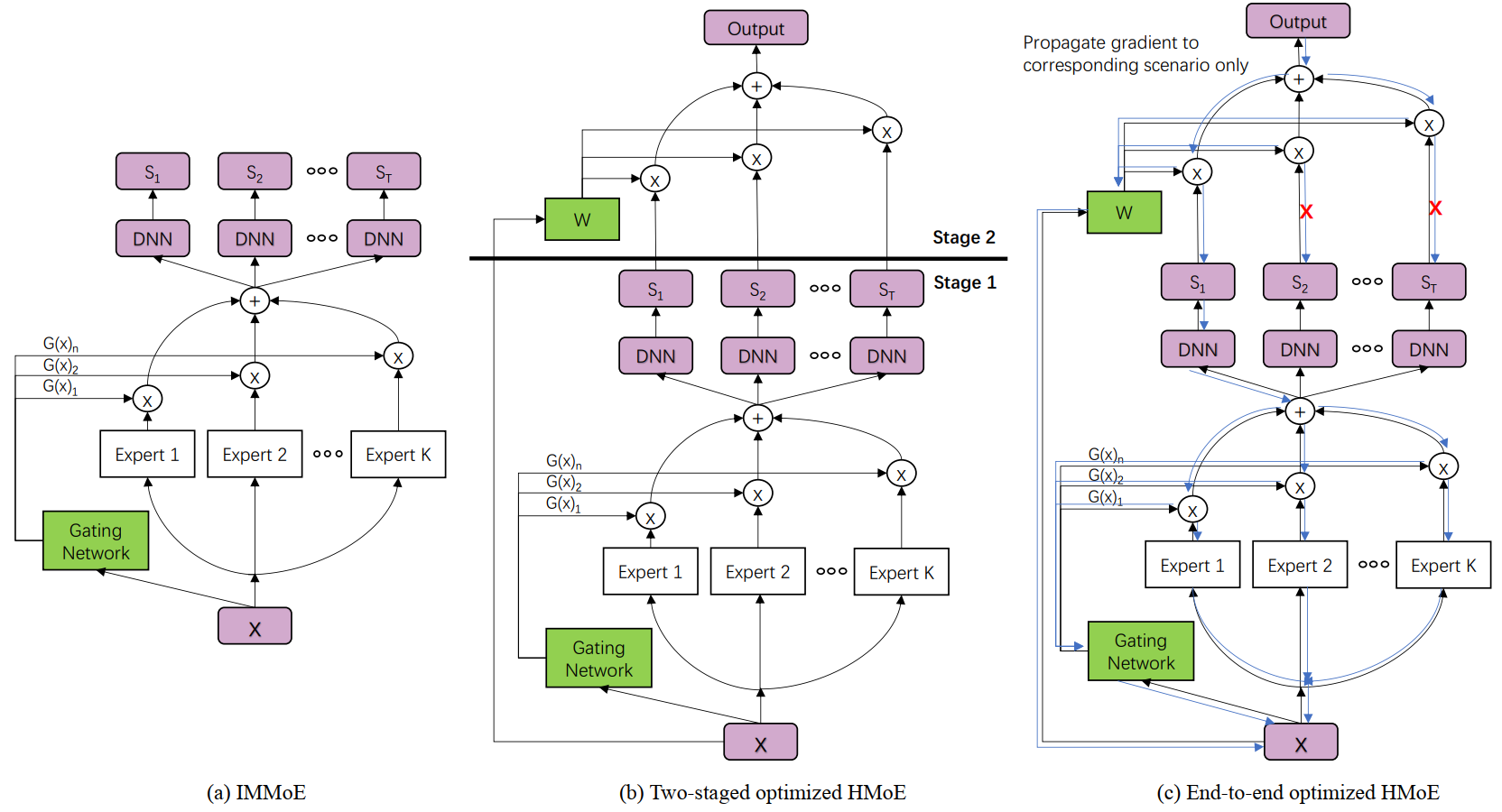
Combination of All above (self research)