TRPO can be viewed as a combination of natural policy gradient, line search strategy and monotonic improvement theorem, it updates policies by taking the largest step possible to improve performance, while satisfying a special constraint on how close the new and old policies are allowed to be. The constraint is expressed in terms of KL-Divergence, a measure of (something like, but not exactly) distance between probability distributions. we will walk through the derivation process and details in the following section.
1. Overview
Just keep in mind: TRPO= NPG + Linesearch + monotonic improvement theorem!
2. Fromulation
STEP1: Problems Setup
Two approaches of writing reward function:
Approach 1: Expected Discounted Reward
(1) The objective function to optimize:
![\[\eta \left( {\rm{\pi }} \right) = {\mathbb{E}_{{s_0},{a_0}, \ldots }}\left[ {\sum\limits_{t = 0}^\infty {{\gamma ^t}r\left( {{s_t}} \right)} } \right]\]](http://www.liaoyong.net/wp-content/ql-cache/quicklatex.com-fc1f9f834c2fee1621913e93a477d7c6_l3.png "Rendered by QuickLaTeX.com")
 .
.Can we express the expected return of another policy in terms of the advantage over the original policy?
(2) Yes, it is proven and shown that a guaranteed increase in the performance is possible.
Approach 2:Compute the reward of a policy using another policy
![\[\eta \left( {{\rm{\tilde \pi }}} \right) = \eta \left( {\rm{\pi }} \right) + {\mathbb{E}_{{s_0},{a_0}, \ldots \sim {\rm{\tilde \pi }}}}\left[ {\sum\limits_{t = 0}^\infty {{\gamma ^t}{A_{\rm{\pi }}}\left( {{s_t},{a_t}} \right)} } \right] = \eta \left( {\rm{\pi }} \right) + \sum\limits_s {{\rho _{{\rm{\tilde \pi }}}}\left( s \right)} \sum\limits_a {{\rm{\tilde \pi }}\left( {a\left| s \right.} \right)} {A_{\rm{\pi }}}\left( {{s_t},{a_t}} \right)\]](http://www.liaoyong.net/wp-content/ql-cache/quicklatex.com-66689227879221f11826f5136fd2d5c7_l3.png "Rendered by QuickLaTeX.com")
 ,
,  can be viewed as the expected return of policy in terms of the advantage over
  , which is the old policy.
 You might wonder why advantage is used. Intuitively, you can think of it as measuring how good the new policy is with regard to the average performance of the old policy.
 of the new policy can be rewrite into the following form, where
  is the (unormalized) discounted visitation frequencies where
![\[\begin{array}{l}\eta \left( {{\rm{\tilde \pi }}} \right) = \eta \left( {\rm{\pi }} \right) + \sum\limits_{t = 0}^\infty {\sum\limits_s {P\left( {{s_t} = s\left| {{\rm{\tilde \pi }}} \right.} \right)} \sum\limits_a {{\rm{\tilde \pi }}\left( {a\left| s \right.} \right)} {\gamma ^t}{A_{\rm{\pi }}}\left( {s,a} \right)} \\{\kern 1pt} {\kern 1pt} {\kern 1pt} {\kern 1pt} {\kern 1pt} {\kern 1pt} {\kern 1pt} {\kern 1pt} {\kern 1pt} {\kern 1pt} {\kern 1pt} {\kern 1pt} {\kern 1pt} {\kern 1pt} {\kern 1pt} {\kern 1pt} {\kern 1pt} {\kern 1pt} {\kern 1pt} {\kern 1pt} {\kern 1pt} {\kern 1pt} {\kern 1pt} {\kern 1pt} {\kern 1pt} {\kern 1pt} {\kern 1pt} = \eta \left( {\rm{\pi }} \right) + \sum\limits_s {\sum\limits_{t = 0}^\infty {{\gamma ^t}P\left( {{s_t} = s\left| {{\rm{\tilde \pi }}} \right.} \right)} } \sum\limits_a {{\rm{\tilde \pi }}\left( {a\left| s \right.} \right)} {A_{\rm{\pi }}}\left( {s,a} \right)\\{\kern 1pt} {\kern 1pt} {\kern 1pt} {\kern 1pt} {\kern 1pt} {\kern 1pt} {\kern 1pt} {\kern 1pt} {\kern 1pt} {\kern 1pt} {\kern 1pt} {\kern 1pt} {\kern 1pt} {\kern 1pt} {\kern 1pt} {\kern 1pt} {\kern 1pt} {\kern 1pt} {\kern 1pt} {\kern 1pt} {\kern 1pt} {\kern 1pt} {\kern 1pt} {\kern 1pt} {\kern 1pt} {\kern 1pt} {\kern 1pt} = \eta \left( {\rm{\pi }} \right) + \sum\limits_s {{\rho _{{\rm{\tilde \pi }}}}\left( s \right)} \sum\limits_a {{\rm{\tilde \pi }}\left( {a\left| s \right.} \right)} {A_{\rm{\pi }}}\left( {s,a} \right)\end{array}\]](http://www.liaoyong.net/wp-content/ql-cache/quicklatex.com-9b04373ff2fba7fb66daf2b0cb38daaf_l3.png "Rendered by QuickLaTeX.com")
![\[{\rho _{\rm{\pi }}}\left( s \right) = P\left( {{s_0} = s} \right) + \gamma P\left( {{s_1} = s} \right) + {\gamma ^2}P\left( {{s_2} = s} \right) + \cdots \]](http://www.liaoyong.net/wp-content/ql-cache/quicklatex.com-88dea452b4c173c287e13f61212b93b4_l3.png "Rendered by QuickLaTeX.com")
is highly dependent on the new policy . However, we can make an approximation to with 
(3) Make an approximation to
to remove the dependency of discounted visitation frequencies under the new policy.The local approximation:
![\[\begin{array}{l}{L_{\rm{\pi }}}\left( {{\rm{\tilde \pi }}} \right) = \eta \left( {\rm{\pi }} \right) + \sum\limits_s {{\rho _{\rm{\pi }}}\left( s \right)} \sum\limits_a {{\rm{\tilde \pi }}\left( {a\left| s \right.} \right)} {A_{\rm{\pi }}}\left( {s,a} \right)\\{L_{{{\rm{\pi }}_{{\theta _0}}}}}\left( {{{\rm{\pi }}_{{\theta _0}}}} \right) = \eta \left( {{{\rm{\pi }}_{{\theta _0}}}} \right)\\{\nabla _\theta }{L_{{{\rm{\pi }}_{{\theta _0}}}}}\left( {{{\rm{\pi }}_\theta }} \right)\left| {_{\theta = {\theta _0}}} \right. = {\nabla _\theta }\eta \left( {{{\rm{\pi }}_\theta }} \right)\left| {_{\theta = {\theta _0}}} \right.\end{array}\]](http://www.liaoyong.net/wp-content/ql-cache/quicklatex.com-de6f0a1e35639e3de71e2d8928e3bf2b_l3.png "Rendered by QuickLaTeX.com")
 with
with  , assuming state visitation frequency is not too different for the new and the old policies.
  uses the visitation frequency rather than , that is, we ignore the changes in state visitation frequency due to the change in policy. To put it in simple terms, we assume that the state visitation frequency is not different for both the new and old policy. When we are calculating the gradient of , which will also improve with respect to some parameter
  we can’t be sure how much big of a step to take.
Kakade and Langford proposed a new policy update method called conservative policy iteration, shown as follows: (CPI (https://arxiv.org/pdf/1509.02971.pdf))
![\[{{\rm{\pi }}_{new}}\left( {a\left| s \right.} \right) = \left( {1 - \alpha } \right){{\rm{\pi }}_{old}}\left( {a\left| s \right.} \right) + \alpha {\rm{\pi '}}\left( {a\left| s \right.} \right)\]](http://www.liaoyong.net/wp-content/ql-cache/quicklatex.com-44cfc73e9bbd9df6617ed191b970db36_l3.png "Rendered by QuickLaTeX.com")
 is the new policy,
  is the old policy, and
  is the policy which maximizes
  , namely,
Kakade and Langford derived the following equation from above equation as follows (Let’s use Theorem 1 to denote it). (Theorem 1 (https://arxiv.org/pdf/1509.02971.pdf))
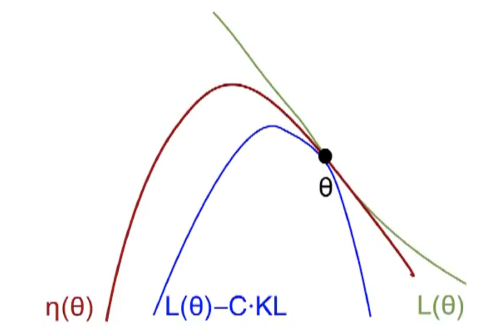
![\[\eta \left( {{\rm{\tilde \pi }}} \right) \ge {L_{\rm{\pi }}}\left( {{\rm{\tilde \pi }}} \right) - CD_{KL}^{\max }\left( {{\rm{\pi }},{\rm{\tilde \pi }}} \right)\]](http://www.liaoyong.net/wp-content/ql-cache/quicklatex.com-586ea23d97b9e059880ae651907f4a35_l3.png "Rendered by QuickLaTeX.com")

 represents the penalty coefficient, whereas
  denotes the maximum KL divergence of the two parameter for each of the state. The concept of KL divergence was originated from information theory, describing the information loss. Simply put, you can view it as how different these two parameters, and are.
(4) Find the lower-bound that guarantees the improvement using MM
The above formula implies that the expected long-term reward η is monotonically improving as long as the right-hand-side term is maximized. Why? Let’s define the right-hand-side of the inequality to be
 . (https://arxiv.org/pdf/1509.02971.pdf)
 ![\[{M_i}\left( {\rm{\pi }} \right) = {L_{{{\rm{\pi }}_i}}}\left( {\rm{\pi }} \right) - CD_{KL}^{\max }\left( {{{\rm{\pi }}_i},{\rm{\pi }}} \right)\]](http://www.liaoyong.net/wp-content/ql-cache/quicklatex.com-cfed4ca9263506d8714d6b85b30d28f2_l3.png "Rendered by QuickLaTeX.com")
![\[\begin{array}{l}\eta \left( {{{\rm{\pi }}_{i + 1}}} \right) \ge {M_i}\left( {{{\rm{\pi }}_{i + 1}}} \right)\\\eta \left( {{{\rm{\pi }}_i}} \right) = {M_i}\left( {{{\rm{\pi }}_i}} \right)\end{array}\]](http://www.liaoyong.net/wp-content/ql-cache/quicklatex.com-8b7d49644965e678f66383c0919ca452_l3.png "Rendered by QuickLaTeX.com")
![\[\eta \left( {{{\rm{\pi }}_{i + 1}}} \right) - \eta \left( {{{\rm{\pi }}_i}} \right) \ge {M_i}\left( {{{\rm{\pi }}_{i + 1}}} \right) - {M_i}\left( {{{\rm{\pi }}_i}} \right)\]](http://www.liaoyong.net/wp-content/ql-cache/quicklatex.com-d01b732ecee7e8aa3d491c0b6da6d2e3_l3.png "Rendered by QuickLaTeX.com")
 . Namely,
 ![\[\mathop {{\rm{maximize}}}\limits_\theta \left[ {{L_{{\theta _{old}}}}\left( \theta \right) - CD_{KL}^{\max }\left( {{\theta _{old}},\theta } \right)} \right]\]](http://www.liaoyong.net/wp-content/ql-cache/quicklatex.com-b7d0bec01917ae4d28926c322e35b065_l3.png "Rendered by QuickLaTeX.com")
with  :
: More explanation from (reference …) is better for understanding:
a) In practice, if penalty coefficient is included in the objective function, the step size will be very small, leading to long training time. Consequently, a constraint on the KL divergence is used to allow a larger step size while guarantee robust performance.
b) But having a penalty coefficient
in the preceding equation will cause the step size to be very small, which in turn slows down the updates. So, we impose a constraint on the KL divergence’s old policy and new policy, which is the trust region constraint, and it will help us to find the optimal step size.c) In practice, if we use the penalty coefficient
recommended by the theory above, the step sizes would be very small. One way to take larger steps in a robust way is to use a constraint on the KL divergence between the new policy and the old policy, i.e., a trust region constraint. Use the average KL instead of the maximum of the KL (heuristic approximation) ![\[\begin{array}{l}\mathop {{\rm{maximize}}}\limits_\theta {L_{{\theta _{old}}}}\left( \theta \right)\\{\rm{subject}}{\kern 1pt} {\kern 1pt} {\kern 1pt} {\rm{to}}{\kern 1pt} {\kern 1pt} {\kern 1pt} {\kern 1pt} D_{KL}^{\max }\left( {{\theta _{old}},\theta } \right) \le \delta \end{array}\]](http://www.liaoyong.net/wp-content/ql-cache/quicklatex.com-637597d29ede587212922af0f65b9c3f_l3.png "Rendered by QuickLaTeX.com")
 . Unfortunately, it is not solvable as there are a infinitely large number of states. The paper proposed a solution which provides a heuristic approximation with the expected KL divergence over states, as opposed to finding the maximum KL divergence. (KL Divergence With State Visitation Frequency )
 ![\[\bar D_{KL}^\rho \left( {{\theta _1},{\theta _2}} \right) \buildrel\textstyle.\over= {E_{s \sim \rho }}\left[ {{D_{KL}}\left( {{{\rm{\pi }}_{{\theta _1}}}\left( { \cdot \left| s \right.} \right)\left\| {{{\rm{\pi }}_{{\theta _2}}}\left( { \cdot \left| s \right.} \right)} \right.} \right)} \right]\]](http://www.liaoyong.net/wp-content/ql-cache/quicklatex.com-538004067b7bd08d41f9e76924103195_l3.png "Rendered by QuickLaTeX.com")
![\[\begin{array}{l}\mathop {{\rm{maximize}}}\limits_\theta {L_{{\theta _{old}}}}\left( \theta \right)\\{\rm{subject}}{\kern 1pt} {\kern 1pt} {\kern 1pt} {\rm{to}}{\kern 1pt} {\kern 1pt} {\kern 1pt} {\kern 1pt} \bar D_{KL}^{{\rho _{{\theta _{old}}}}}\left( {{\theta _{old}},\theta } \right) \le \delta \end{array}\]](http://www.liaoyong.net/wp-content/ql-cache/quicklatex.com-658816eb617301755bf5b5d1b773f63b_l3.png "Rendered by QuickLaTeX.com")
![\[\begin{array}{l}\mathop {{\rm{maximize}}}\limits_\theta \sum\limits_s {{\rho _{{\theta _{old}}}}\left( s \right)} \sum\limits_a {{{\rm{\pi }}_\theta }\left( {a\left| s \right.} \right)} {A_{{\theta _{old}}}}\left( {s,a} \right)\\{\rm{subject}}{\kern 1pt} {\kern 1pt} {\kern 1pt} {\rm{to}}{\kern 1pt} {\kern 1pt} {\kern 1pt} {\kern 1pt} \bar D_{KL}^{{\rho _{{\theta _{old}}}}}\left( {{\theta _{old}},\theta } \right) \le \delta \end{array}\]](http://www.liaoyong.net/wp-content/ql-cache/quicklatex.com-218a535bd6606da14c26b30c668a7e36_l3.png "Rendered by QuickLaTeX.com")
Now replace sum over states
 as expectation
  and replace sum over actions by important sampling estimator as
 ![\[\sum\limits_a {{{\rm{\pi }}_\theta }\left( {a\left| s \right.} \right)} {A_{{\theta _{old}}}}\left( {s,a} \right) = {\mathbb{E}_{a \sim q}}\left[ {\frac{{{{\rm{\pi }}_\theta }\left( {a\left| s \right.} \right)}}{{q\left( {a\left| s \right.} \right)}}{A_{{\theta _{old}}}}\left( {s,a} \right)} \right]\]](http://www.liaoyong.net/wp-content/ql-cache/quicklatex.com-46d6979c63fbf58e8d4eb580bba281f4_l3.png "Rendered by QuickLaTeX.com")
![\[\begin{array}{l}\mathop {{\rm{maximize}}}\limits_\theta {\mathbb{E}_{s \sim {{\rm{\pi }}_{{\theta _{old}}}},a \sim {{\rm{\pi }}_{{\theta _{old}}}}}}\left[ {\frac{{{{\rm{\pi }}_\theta }\left( {a\left| s \right.} \right)}}{{{{\rm{\pi }}_{{\theta _{old}}}}\left( {a\left| s \right.} \right)}}{A_{{\theta _{old}}}}\left( {s,a} \right)} \right]\\{\rm{subject}}{\kern 1pt} {\kern 1pt} {\kern 1pt} {\rm{to}}{\kern 1pt} {\kern 1pt} {\kern 1pt} {\kern 1pt} {\mathbb{E}_{s \sim {{\rm{\pi }}_{{\theta _{old}}}}}}\left[ {{D_{KL}}\left( {{{\rm{\pi }}_{{\theta _{old}}}}\left( { \cdot \left| s \right.} \right)\left\| {{{\rm{\pi }}_\theta }\left( { \cdot \left| s \right.} \right)} \right.} \right)} \right] \le \delta \end{array}\]](http://www.liaoyong.net/wp-content/ql-cache/quicklatex.com-454e0eea44b07f4a167abb1101716661_l3.png "Rendered by QuickLaTeX.com")
STEP2:Problem Solving
(6) Using line-search (Approximation, Fisher matrix, Conjugate gradient)
The loss function is defined as
![\[L\left( {\rm{\pi }} \right) = {\mathbb{E}_{\tau \sim {{\rm{\pi }}_k}}}\left[ {\sum\limits_{t = 0}^\infty {{\gamma ^t}\frac{{{\rm{\pi }}\left( {{a_t}\left| {{s_t}} \right.} \right)}}{{{{\rm{\pi }}_k}\left( {{a_t}\left| {{s_t}} \right.} \right)}}{A^{\rm{\pi }}}\left( {{s_t},{a_t}} \right)} } \right]\]](http://www.liaoyong.net/wp-content/ql-cache/quicklatex.com-0cf8c7178f9690018e2771212edef1ff_l3.png "Rendered by QuickLaTeX.com")
 should be easy to optimize. In fact, we approximate and the mean of the KL-divergence using Taylor Series up to the first order for and second order for the KL-divergence:
 ![\[\begin{array}{l}{L_{{\theta _k}}}\left( \theta \right) \approx {L_{{\theta _k}}}\left( {{\theta _k}} \right) + {g^T}\left( {\theta - {\theta _k}} \right) + \ldots \\{{\bar D}_{KL}}\left( {\theta \left\| {{\theta _k}} \right.} \right) \approx {{\bar D}_{KL}}\left( {{\theta _k}\left\| {{\theta _k}} \right.} \right) + {\nabla _\theta }{{\bar D}_{KL}}\left( {\theta \left\| {{\theta _k}} \right.} \right)\left| {_{{\theta _k}}} \right.\left( {\theta - {\theta _k}} \right) + \frac{1}{2}{\left( {\theta - {\theta _k}} \right)^T}H\left( {\theta - {\theta _k}} \right)\end{array}\]](http://www.liaoyong.net/wp-content/ql-cache/quicklatex.com-cd667ada07c2a4ee34c62c674c67430d_l3.png "Rendered by QuickLaTeX.com")
![\[\begin{array}{l}{L_{{\theta _k}}}\left( \theta \right) \approx {g^T}\left( {\theta - {\theta _k}} \right){\kern 1pt} {\kern 1pt} {\kern 1pt} {\kern 1pt} {\kern 1pt} {\kern 1pt} {\kern 1pt} {\kern 1pt} {\kern 1pt} {\kern 1pt} {\kern 1pt} {\kern 1pt} {\kern 1pt} {\kern 1pt} {\kern 1pt} {\kern 1pt} {\kern 1pt} {\kern 1pt} {\kern 1pt} {\kern 1pt} {\kern 1pt} {\kern 1pt} {\kern 1pt} {\kern 1pt} {\kern 1pt} {\kern 1pt} {\kern 1pt} {\kern 1pt} {\kern 1pt} {\kern 1pt} {\kern 1pt} {\kern 1pt} {\kern 1pt} {\kern 1pt} {\kern 1pt} {\kern 1pt} {\kern 1pt} {\kern 1pt} {\kern 1pt} {\kern 1pt} {\kern 1pt} {\kern 1pt} {\kern 1pt} {\kern 1pt} {\kern 1pt} {\kern 1pt} {\kern 1pt} {\kern 1pt} {\kern 1pt} {\kern 1pt} {\kern 1pt} {\kern 1pt} {\kern 1pt} {\kern 1pt} {\kern 1pt} {\kern 1pt} {\kern 1pt} {\kern 1pt} {\kern 1pt} {\kern 1pt} {\kern 1pt} {\kern 1pt} {\kern 1pt} {\kern 1pt} {\kern 1pt} {\kern 1pt} {\kern 1pt} {\kern 1pt} {\kern 1pt} {\kern 1pt} {\kern 1pt} {\kern 1pt} {\kern 1pt} {\kern 1pt} {\kern 1pt} {\kern 1pt} {\kern 1pt} {\kern 1pt} {\kern 1pt} {\kern 1pt} {\kern 1pt} {\kern 1pt} {\kern 1pt} g \buildrel\textstyle.\over= {\nabla _\theta }{L_{{\theta _k}}}\left( \theta \right)\left| {_{{\theta _k}}} \right.\\{{\bar D}_{KL}}\left( {\theta \left\| {{\theta _k}} \right.} \right) \approx \frac{1}{2}{\left( {\theta - {\theta _k}} \right)^T}H\left( {\theta - {\theta _k}} \right){\kern 1pt} {\kern 1pt} {\kern 1pt} {\kern 1pt} {\kern 1pt} {\kern 1pt} {\kern 1pt} {\kern 1pt} {\kern 1pt} {\kern 1pt} {\kern 1pt} {\kern 1pt} H \buildrel\textstyle.\over= \nabla _\theta ^2{{\bar D}_{KL}}\left( {\theta \left\| {{\theta _k}} \right.} \right)\left| {_{{\theta _k}}} \right.\end{array}\]](http://www.liaoyong.net/wp-content/ql-cache/quicklatex.com-749ffde28355af9af48161950526a4b3_l3.png "Rendered by QuickLaTeX.com")
 is the policy gradient and
  is called the Fisher Information matrix FIM in the form of a Hessian matrix.
 ![\[H = {\nabla ^2}f = \left( {\begin{array}{*{20}{c}}{\frac{{{\partial ^2}f}}{{\partial x_1^2}}}&{\frac{{{\partial ^2}f}}{{\partial {x_1}\partial {x_2}}}}& \cdots &{\frac{{{\partial ^2}f}}{{\partial {x_1}\partial {x_n}}}}\\{\frac{{{\partial ^2}f}}{{\partial {x_2}\partial {x_1}}}}&{\frac{{{\partial ^2}f}}{{\partial x_2^2}}}& \cdots &{\frac{{{\partial ^2}f}}{{\partial {x_2}\partial {x_n}}}}\\\vdots & \vdots & \ddots & \vdots \\{\frac{{{\partial ^2}f}}{{\partial {x_n}\partial {x_1}}}}&{\frac{{{\partial ^2}f}}{{\partial {x_n}\partial {x_2}}}}& \cdots &{\frac{{{\partial ^2}f}}{{\partial x_n^2}}}\end{array}} \right)\]](http://www.liaoyong.net/wp-content/ql-cache/quicklatex.com-b8ce1650d4a15455932062c01c3b0195_l3.png "Rendered by QuickLaTeX.com")
![\[\begin{array}{l}{\theta _{k + 1}} = \mathop {\arg \max }\limits_\theta {g^T}\left( {\theta - {\theta _k}} \right){\kern 1pt} {\kern 1pt} \\s.t.{\kern 1pt} {\kern 1pt} {\kern 1pt} {\kern 1pt} {\kern 1pt} {\kern 1pt} {\kern 1pt} \frac{1}{2}{\left( {\theta - {\theta _k}} \right)^T}H\left( {\theta - {\theta _k}} \right){\kern 1pt} {\kern 1pt} {\kern 1pt} {\kern 1pt} \le \delta \end{array}\]](http://www.liaoyong.net/wp-content/ql-cache/quicklatex.com-81657a398f8bb514eeec00977b20f7f8_l3.png "Rendered by QuickLaTeX.com")
![\[{\theta _{k + 1}} = {\theta _k} + \sqrt {\frac{{2\delta }}{{{g^T}{H^{ - 1}}g}}} {H^{ - 1}}g\]](http://www.liaoyong.net/wp-content/ql-cache/quicklatex.com-0b8b084c2d1f17f7d4e5889914108450_l3.png "Rendered by QuickLaTeX.com")
 by solving
  for the following linear equation:
 ![\[\begin{array}{l}{x_k} \approx \hat H_k^{ - 1}{{\hat g}_k}\\{{\hat H}_k}{x_k} \approx {{\hat g}_k}\end{array}\]](http://www.liaoyong.net/wp-content/ql-cache/quicklatex.com-45d53f1812524c2b1ea706ab9c86d100_l3.png "Rendered by QuickLaTeX.com")
It turns out we can solve it with the conjugate gradient method which is computational less complex than finding the inverse of
. Conjugate gradient is similar to gradient descent but it can find the optimal point in at most N iterations where N is the number of parameters in the model.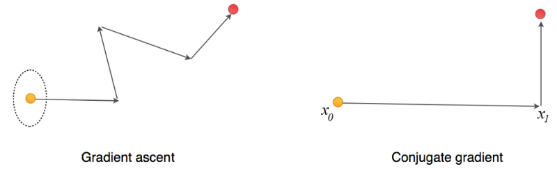
3. Pseudocode
OpenAI Spiningup version: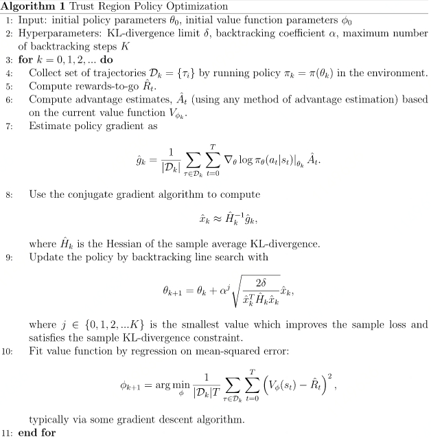
4. Implementation
This code implementation is modified from original git, I include everything into a single file to facilitate its implementation and understanding.
|
1 2 3 4 5 6 7 8 9 10 11 12 13 14 15 16 17 18 19 20 21 22 23 24 25 26 27 28 29 30 31 32 33 34 35 36 37 38 39 40 41 42 43 44 45 46 47 48 49 50 51 52 53 54 55 56 57 58 59 60 61 62 63 64 65 66 67 68 69 70 71 72 73 74 75 76 77 78 79 80 81 82 83 84 85 86 87 88 89 90 91 92 93 94 95 96 97 98 99 100 101 102 103 104 105 106 107 108 109 110 111 112 113 114 115 116 117 118 119 120 121 122 123 124 125 126 127 128 129 130 131 132 133 134 135 136 137 138 139 140 141 142 143 144 145 146 147 148 149 150 151 152 153 154 155 156 157 158 159 160 161 162 163 164 165 166 167 168 169 170 171 172 173 174 175 176 177 178 179 180 181 182 183 184 185 186 187 188 189 190 191 192 193 194 195 196 197 198 199 200 201 202 203 204 205 206 207 208 209 210 211 212 213 214 215 216 217 218 219 220 221 222 223 224 225 226 227 228 229 230 231 232 233 234 235 236 237 238 239 240 241 242 243 244 245 246 247 248 249 250 251 252 253 254 255 256 257 258 259 260 261 262 263 264 265 266 267 268 269 270 271 272 273 274 275 276 277 278 279 280 281 282 283 284 285 286 287 288 289 290 291 292 293 294 295 296 297 298 299 300 301 302 303 304 305 306 307 308 309 310 311 312 313 314 315 316 317 318 319 320 321 322 323 324 325 326 327 328 329 330 331 332 333 334 335 336 337 338 339 340 341 342 343 344 345 346 347 348 349 350 351 352 353 354 355 356 357 358 359 360 361 362 363 364 365 366 367 368 369 370 371 372 373 374 375 376 377 378 379 380 381 382 383 384 385 386 387 388 389 390 391 392 393 394 395 396 397 398 399 400 401 402 403 404 405 406 407 408 409 410 411 412 413 414 415 416 417 418 419 420 |
import tensorflow as tf import numpy as np import scipy.signal from gym.spaces import Box, Discrete import gym EPS = 1e-8 def combined_shape(length, shape=None): #return tuple type if shape is None: return (length, ) return (length, shape) if np.isscalar(shape) else (length, *shape) def placeholder(dim=None): return tf.placeholder(dtype=tf.float32, shape=combined_shape(None, dim)) def placeholders(*args): return [placeholder(dim) for dim in args] # print(combined_shape(None, shape=3)) # (None, 3) # print(placeholder(dim=3)) # Tensor("Placeholder:0", shape=(?, 3), dtype=float32) # print(placeholders((3,3,3))) # [<tf.Tensor 'Placeholder_1:0' shape=(?, 3, 3, 3) dtype=float32>] def placeholder_from_space(space): if isinstance(space, Box): return placeholder(space.shape) elif isinstance(space, Discrete): return tf.placeholder(dtype=tf.int32, shape=(None, )) raise NotImplementedError def placeholder_from_spaces(*args): return [placeholder_from_space(space) for space in args] #return single list def keys_as_sorted_list(dict): return sorted(list(dict.keys())) def values_as_sorted_list(dict): return [dict[k] for k in keys_as_sorted_list(dict)] def flat_concat(xs): return tf.concat([tf.reshape(x, (-1,)) for x in xs], axis=0) def flat_grad(f, params): return flat_concat(tf.gradients(xs=params, ys=f)) def get_vars(scope=''): return [x for x in tf.trainable_variables() if scope in x.name] def count_vars(scope=''): v = get_vars(scope) return sum([np.prod(var.shape.as_list()) for var in v]) def hessian_vector_product(f, params): # for H = grad**2 f, compute Hx g = flat_grad(f, params) x = tf.placeholder(tf.float32, shape=g.shape) return x, flat_grad(tf.reduce_sum(g*x),params) def assign_params_from_flat(x, params): flat_size = lambda p : int(np.prod(p.shape.as_list())) # the 'int' is important for scalars splits = tf.split(x, [flat_size(p) for p in params]) new_params = [tf.reshape(p_new, p.shape) for p, p_new in zip(params, splits)] return tf.group([tf.assign(p, p_new) for p, p_new in zip(params, new_params)]) def mlp(x, hidden_sizes=(32,), activation=tf.tanh, output_activation=None): for h in hidden_sizes[:-1]: x = tf.layers.dense(x, units=h, activation=activation) return tf.layers.dense(x, hidden_sizes[-1], activation=output_activation) def guassian_likelihood(x, mu, log_std): pre_sum = -0.5 * (((x-mu)/(tf.exp(log_std)+EPS))**2 + 2*log_std + np.log(2*np.pi)) return tf.reduce_sum(pre_sum, axis=1) def diagonal_guassian_kl(mu0, log_std0, mu1, log_std1): """tf symbol for mean KL divergence between two batches of diagonal gaussian distributions, where distributions are specified by means and log stds.""" var0, var1 = tf.exp(2 * log_std0), tf.exp(2 * log_std1) pre_sum = 0.5 * (((mu1-mu0)**2 + var0)/(var1 + EPS) - 1) + log_std1 - log_std0 all_kls = tf.reduce_sum(pre_sum, axis=1) return tf.reduce_mean(all_kls) def categorical_kl(logp0, logp1): """tf symbol for mean KL divergence between two batches of categorical probability distributions, where the distributions are input as log probs.""" all_kls = tf.reduce_sum(tf.exp(logp1) * (logp1 - logp0), axis=1) return tf.reduce_mean(all_kls) def discount_cumsum(x, discount): """ input: vector x, [x0, x1, x2] output: [x0 + discount*x1 + discount^2*x2, x1 + discount*x2, x2] """ return scipy.signal.lfilter([1], [1, float(-discount)], x[::-1], axis=0)[::-1] def x_sum(x): x, scalar = ([x], True) if np.isscalar(x) else (x, False) buff = np.asarray(x, dtype=np.float32) return x if scalar else buff def statistics_scalar(x, with_min_and_max=False): x = np.array(x, dtype=np.float32) x_sum, x_n = [np.sum(x), len(x)] mean = x_sum / x_n x_sum_sq = np.sum((x-mean)**2) std = np.sqrt(x_sum_sq/x_n) if with_min_and_max: x_min = np.min(x) if len(x)>0 else np.inf x_max = np.max(x) if len(x)>0 else -np.inf return mean, std, x_min, x_max return mean, std def mlp_categorical_policy(x, a, hidden_sizes, activation, output_activation, action_space): act_dim = action_space.n # type int, val:2 logits = mlp(x, list(hidden_sizes)+[act_dim], activation, None) #concatenate list; shape=(?, 2), dtype=float32 logp_all = tf.nn.log_softmax(logits) #shape=(?, 2), dtype=float32 # print(tf.multinomial(logits, 1)) #shape=(?, 1), dtype=int64, sample one sample pi = tf.squeeze(tf.multinomial(logits, 1), axis=1) #shape=(?,), dtype=int64 logp = tf.reduce_sum(tf.one_hot(a, depth=act_dim) * logp_all, axis=1) #shape=(?,), dtype=float32 logp_pi = tf.reduce_sum(tf.one_hot(pi, depth=act_dim) * logp_all, axis=1) #shape=(?,), dtype=float32 old_logp_all = placeholder(act_dim) # shape=(?, 2), dtype=float32 d_kl = categorical_kl(logp_all, old_logp_all) #shape=(), dtype=float32 info = {'logp_all':logp_all} #shape=(?, 2) dtype=float32 info_phs = {'logp_all': old_logp_all} #shape=(?, 2) dtype=float32> return pi, logp, logp_pi, info, info_phs, d_kl def mlp_gaussian_policy(x, a, hidden_sizes, activation, output_activation, action_space): act_dim = a.shape.as_list()[-1] mu = mlp(x, list(hidden_sizes)+[act_dim], activation, output_activation) log_std = tf.get_variable(name='log_std', initializer=-0.5*np.ones(act_dim, dtype=np.float32)) std = tf.exp(log_std) pi = mu + tf.random_normal(tf.shape(mu)) * std logp = guassian_likelihood(a, mu, log_std) logp_pi = guassian_likelihood(pi, mu, log_std) old_mu_ph, old_log_std_ph = placeholders(act_dim, act_dim) d_kl = diagonal_guassian_kl(mu, log_std, old_mu_ph, old_log_std_ph) info = {'mu':mu, 'log_std':log_std} info_phs = {'mu':old_mu_ph, 'log_std':old_log_std_ph} return pi, logp, logp_pi, info, info_phs, d_kl def mlp_actor_critic(x, a, hidden_sizes=(64,64), activation=tf.tanh, output_activation=None, policy=None, action_space=None): # default policy builder depends on action space if policy is None and isinstance(action_space, Box): policy = mlp_gaussian_policy elif policy is None and isinstance(action_space, Discrete): policy = mlp_categorical_policy with tf.variable_scope('pi'): policy_outs = policy(x, a, hidden_sizes, activation, output_activation, action_space) pi, logp, logp_pi, info, info_phs, d_kl = policy_outs with tf.variable_scope('v'): v = tf.squeeze(mlp(x, list(hidden_sizes)+[1], activation, None), axis=1) return pi, logp, logp_pi, info, info_phs, d_kl, v class GAEBuffer(object): """ A buffer for storing trajectories experienced by a TRPO agent interacting with the environment, and using Generalized Advantage Estimation (GAE-Lambda) for calculating the advantages of state-action pairs. """ def __init__(self, obs_dim, act_dim, size, info_shapes, gamma=0.99, lam=0.95): self.obs_buf = np.zeros(combined_shape(size, obs_dim), dtype=np.float32) self.act_buf = np.zeros(combined_shape(size, act_dim), dtype=np.float32) self.adv_buf = np.zeros(size, dtype=np.float32) self.rew_buf = np.zeros(size, dtype=np.float32) self.ret_buf = np.zeros(size, dtype=np.float32) self.val_buf = np.zeros(size, dtype=np.float32) self.logp_buf = np.zeros(size, dtype=np.float32) self.info_bufs = {k: np.zeros([size] + list(v), dtype=np.float32) for k,v in info_shapes.items()} self.sorted_info_keys = keys_as_sorted_list(self.info_bufs) self.gamma, self.lam = gamma, lam self.ptr, self.ptr_start_idx, self.max_size = 0, 0, size def store(self, obs, act, rew, val, logp, info): """Append one timestep of agent-environment interaction to the buffer.""" assert self.ptr < self.max_size self.obs_buf[self.ptr] = obs self.act_buf[self.ptr] = act self.rew_buf[self.ptr] = rew self.val_buf[self.ptr] = val self.logp_buf[self.ptr] = logp for i, k in enumerate(self.sorted_info_keys): self.info_bufs[k][self.ptr] = info[i] self.ptr += 1 def finish_path(self, last_val=0): #trajectory level """ Call this at the end of a trajectory, or when one gets cut off by an epoch ending. This looks back in the buffer to where the trajectory started, and uses rewards and value estimates from the whole trajectory to compute advantage estimates with GAE-Lambda, as well as compute the rewards-to-go for each state, to use as the targets for the value function. The "last_val" argument should be 0 if the trajectory ended because the agent reached a terminal state (died), and otherwise should be V(s_T), the value function estimated for the last state. This allows us to bootstrap the reward-to-go calculation to account for timesteps beyond the arbitrary episode horizon (or epoch cutoff). """ # a = np.array([1, 2, 3, 4, 5, 6, 7, 8, 9, 10]) # print(slice[2, 6, 1]) # start 2,end 6,step 1 # print(a[slice(2, 6, 1)]) # [3 4 5 6] path_slice = slice(self.ptr_start_idx, self.ptr) #specify how to slice a sequence. rews = np.append(self.rew_buf[path_slice], last_val) vals = np.append(self.val_buf[path_slice], last_val) # the next two lines implement GAE-Lambda advantage calculation deltas = rews[:-1] + self.gamma * vals[1:] - vals[:-1] self.adv_buf[path_slice] = discount_cumsum(deltas, self.gamma*self.lam) # the next line computes rewards-to-go, to be targets for the value function self.ret_buf[path_slice] = discount_cumsum(rews, self.gamma)[:-1] self.ptr_start_idx = self.ptr def get(self): #epoch level """ Call this at the end of an epoch to get all of the data from the buffer, with advantages appropriately normalized (shifted to have mean zero and std one). Also, resets some pointers in the buffer. """ assert self.ptr == self.max_size # buffer has to be full before you can get self.ptr, self.ptr_start_idx = 0, 0 # the next two lines implement the advantage normalization trick adv_mean, adv_std = statistics_scalar(self.adv_buf) self.adv_buf = (self.adv_buf - adv_mean) / adv_std return [self.obs_buf, self.act_buf, self.adv_buf, self.ret_buf, self.logp_buf] + values_as_sorted_list(self.info_bufs) def trpo(env_fn, actor_critic=mlp_actor_critic, ac_kwargs=dict(), steps_per_epoch=4000, epochs=50, gamma=0.99, delta=0.01, vf_lr=1e-3, damping_coeff=0.1, cg_iters=10, seed=0, backtrack_iters=10, backtrack_coeff=0.8, lam=0.97, max_ep_len=1000, algo='trpo',train_v_iters=80): """ Trust Region Policy Optimization (with support for Natural Policy Gradient) Args: env_fn: A function which creates a copy of the environment. The environment must satisfy the OpenAI Gym API. actor_critic: A function which takes in placeholder symbols for state, ``x_ph``, and action, ``a_ph``, and returns the main outputs from the agent's Tensorflow computation graph: ============ ================ ==================================================================== Symbol Shape Description ============ ================ ==================================================================== ``pi`` (batch, act_dim) | Samples actions from policy given states. ``logp`` (batch,) | Gives log probability, according to the policy, of taking actions | ``a_ph`` in states ``x_ph``. ``logp_pi`` (batch,) | Gives log probability, according to the policy, of the action | sampled by``pi``. ``info`` N/A | A dict of any intermediate quantities (from calculating the policy or log | probabilities) which are needed for analytically computing KL divergence. | (eg sufficient statistics of the distributions) ``info_phs`` N/A | A dict of placeholders for old values of the entries in ``info``. ``d_kl`` () | A symbol for computing the mean KL divergence between the current policy | (``pi``) and the old policy (as specified by the inputs to ``info_phs``) | over the batch of states given in ``x_ph``. ``v`` (batch,) | Gives the value estimate for states in ``x_ph``. (Critical: make sure | to flatten this!) ============ ================ ==================================================================== ac_kwargs (dict): Any kwargs appropriate for the actor_critic function you provided to TRPO. steps_per_epoch:(int): Number of steps of interaction (state-action pairs) for the agent and the environment in each epoch. epochs (int): Number of epochs of interaction (equivalent to number of policy updates) to perform. gamma (float): Discount factor. (Always between 0 and 1.) delta (float): KL-divergence limit for TRPO / NPG update. (Should be small for stability. Values like 0.01, 0.05.) vf_lr (float): Learning rate for value function optimizer. damping_coeff: (float): Artifact for numerical stability, should be smallish. Adjusts Hessian-vector product calculation: .. math:: Hv \\rightarrow (\\alpha I + H)v where :math:`\\alpha` is the damping coefficient. Probably don't play with this hyperparameter. cg_iters (int): Number of iterations of conjugate gradient to perform. Increasing this will lead to a more accurate approximation to :math:`H^{-1} g`, and possibly slightly-improved performance, but at the cost of slowing things down. Also probably don't play with this hyperparameter. seed (int): Seed for random number generators. backtrack_iters (int): Maximum number of steps allowed in the backtracking line search. Since the line search usually doesn't backtrack, and usually only steps back once when it does, this hyperparameter doesn't often matter. backtrack_coeff (float): How far back to step during backtracking line search. (Always between 0 and 1, usually above 0.5.) lam (float): Lambda for GAE-Lambda. (Always between 0 and 1, close to 1.) max_ep_len (int): Maximum length of trajectory / episode / rollout. algo: Either 'trpo' or 'npg': this code supports both, since they are almost the same. train_v_iters (int): Number of gradient descent steps to take on value function per epoch. """ tf.set_random_seed(seed) np.random.seed(seed) env = env_fn obs_dim = env.observation_space.shape #(4,) act_dim = env.action_space.shape #() # Share information about action space with policy architecture # print(env.action_space) #Discrete(2) ac_kwargs['action_space'] = env.action_space # Inputs to computation graph x_ph, a_ph = placeholder_from_spaces(env.observation_space, env.action_space) # print(x_ph) #shape=(?, 4), dtype=float32) # print(a_ph) #shape=(?,), dtype=int32 adv_ph, ret_ph, logp_old_ph = placeholders(None, None, None) #all with shape=(?,), dtype=float32 # Main outputs from computation graph, plus placeholders for old pdist (for KL) pi, logp, logp_pi, info, info_phs, d_kl, v = actor_critic(x_ph, a_ph, **ac_kwargs) # Need all placeholders in *this* order later (to zip with data from buffer) all_phs = [x_ph, a_ph, adv_ph, ret_ph, logp_old_ph] + values_as_sorted_list(info_phs) # Every step, get: action, value, logprob, & info for pdist (for computing kl div) get_action_ops = [pi, v, logp_pi] + values_as_sorted_list(info) # Experience buffer info_shapes = {k: v.shape.as_list()[1:] for k,v in info_phs.items()} buf = GAEBuffer(obs_dim, act_dim, steps_per_epoch, info_shapes, gamma, lam) # Count variables var_counts = tuple(count_vars(scope) for scope in ['pi', 'v']) print('Numbe of parameters: {}'.format(var_counts)) # TRPO losses ratio = tf.exp(logp - logp_old_ph) # pi(a|s) / pi_old(a|s) pi_loss = - tf.reduce_mean(ratio * adv_ph) v_loss = tf.reduce_mean((ret_ph - v)**2) # Optimizer for value function train_vf = tf.train.AdamOptimizer(learning_rate=vf_lr).minimize(v_loss) # Symbols needed for CG solver pi_params = get_vars('pi') gradient = flat_grad(pi_loss, pi_params) v_ph, hvp = hessian_vector_product(d_kl, pi_params) if damping_coeff > 0: hvp += damping_coeff * v_ph # Symbols for getting and setting params get_pi_params = flat_concat(pi_params) set_pi_params = assign_params_from_flat(v_ph, pi_params) sess = tf.Session() sess.run(tf.global_variables_initializer()) def cg(Ax, b): #Conjugate gradient algorithm x = np.zeros_like(b) r = b.copy() # Note: should be 'b - Ax(x)', but for x=0, Ax(x)=0. Change if doing warm start. p = r.copy() r_dot_old = np.dot(r, r) for _ in range(cg_iters): z = Ax(p) alpha = r_dot_old / (np.dot(p, z) + EPS) x += alpha * p r -= alpha * z r_dot_new = np.dot(r, r) p = r + (r_dot_new / r_dot_old) * p r_dot_old = r_dot_new return x def update(): # Prepare hessian func, gradient eval inputs = {k:v for k,v in zip(all_phs, buf.get())} Hx = lambda x : x_sum(sess.run(hvp, feed_dict={**inputs, v_ph:x})) g, pi_l_old, v_l_old = sess.run([gradient, pi_loss, v_loss], feed_dict=inputs) g, pi_l_old = x_sum(g), x_sum(pi_l_old) # Core calculations for TRPO or NPG x = cg(Hx, g) alpha = np.sqrt(2 * delta /(np.dot(x, Hx(x)) + EPS)) old_params = sess.run(get_pi_params) def set_and_eval(step): sess.run(set_pi_params, feed_dict={v_ph:old_params - alpha * x * step}) return x_sum(sess.run([d_kl, pi_loss], feed_dict=inputs)) if algo == 'npg': # npg has no backtracking or hard kl constraint enforcement kl, pi_l_new = set_and_eval(step=1.) elif algo == 'trpo': # trpo augments npg with backtracking line search, hard kl for j in range(backtrack_iters): kl, pi_l_new = set_and_eval(step=backtrack_coeff ** j) if kl <= delta and pi_l_new <= pi_l_old: print('Accepting new params at step {} of line search.'.format(j)) break if j==backtrack_iters-1: print('Line search failed! Keeping old params.') kl, pi_l_new = set_and_eval(step=0.) # Value function updates for _ in range(train_v_iters): sess.run(train_vf, feed_dict=inputs) v_l_new = sess.run(v_loss, feed_dict=inputs) # Log changes from update print("LossPi={}, LossV={}, KL={}, DeltaLossPi={}, DeltaLassV={}".format( pi_l_old, v_l_old, kl, (pi_l_new - pi_l_old), (v_l_new - v_l_old))) o, r, d, ep_ret, ep_len = env.reset(), 0, False, 0, 0 # Main loop: collect experience in env and update/log each epoch for epoch in range(epochs): for t in range(steps_per_epoch): agent_outs = sess.run(get_action_ops, feed_dict={x_ph: o.reshape(1, -1)}) a, v_t, logp_t, info_t = agent_outs[0][0], agent_outs[1], agent_outs[2], agent_outs[3:] buf.store(o, a, r, v_t, logp_t, info_t) o, r, d, _ = env.step(a) ep_ret += r ep_len += 1 terminal = d or (ep_len == max_ep_len) if terminal or (t==steps_per_epoch-1): if not(terminal): print("Warning: trajectory cut off by epoch at {} steps.".format(ep_len)) # if trajectory didn't reach terminal state, bootstrap value target last_val = r if d else sess.run(v, feed_dict={x_ph: o.reshape(1, -1)}) buf.finish_path(last_val) if terminal: print("EpRet={}, EpLen={}".format(ep_ret,ep_len)) o, r, d, ep_ret, ep_len = env.reset(), 0, False, 0, 0 # Perform TRPO or NPG update! update() if __name__ == '__main__': env = gym.make("CartPole-v1") # env = gym.make("MountainCar-v0") state = env.reset() trpo(env_fn=env, actor_critic=mlp_actor_critic, ac_kwargs=dict(hidden_sizes=[64,64])) |
5.Summary
Again, no more words, just a single graph for summarization as bellow: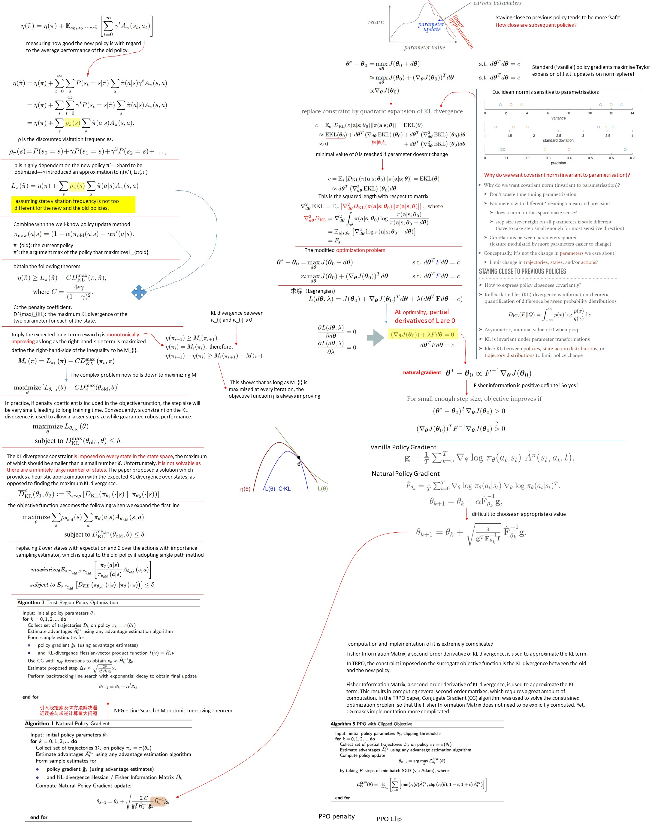
6. Reference
(1). Trust Region Policy Optimization, Schulman et al. 2015
(2). OpenAI Spinningup Documentation-TRPO
(3). rl-proximal-policy-optimization-ppo-explained
(4). rl-the-math-behind-trpo-ppo
(5). introduction-to-various-reinforcement-learning-algorithms-part-ii-trpo-ppo
(6). rl-trust-region-policy-optimization-trpo-explained